Normal Outcome (Known SD) • beastt

Introduction and Data Description

In this example, we illustrate how to use Bayesian dynamic borrowing (BDB) with the inclusion of inverse probability weighting to balance baseline covariate distributions between external and internal datasets. This particular example considers a hypothetical trial with a cross sectional normal outcome and a known standard deviation (SD) in each treatment arm (external control arm and both internal arms), and our objective is to use BDB with IPWs to construct a posterior distribution for the control mean $\theta_C$ . We will use simulated internal and external datasets from the package where each dataset has a normally distributed response variable and four baseline covariates which we will balance.

The external control dataset has a sample size of 150 participants, and the distributions of the four covariates are as follows: - Covariate 1: normal with a mean and standard deviation of approximately 50 and 10, respectively - Covariate 2: binary (0 vs. 1) with approximately 20% of participants with level 1 - Covariate 3: binary (0 vs. 1) with approximately 60% of participants with level 1 - Covariate 4: binary (0 vs. 1) with approximately 30% of participants with level 1

The internal dataset has 120 participants with 60 participants in each of the control and active treatment arms. The covariate distributions of each arm are as follows: - Covariate 1: normal with a mean and standard deviation of approximately 55 and 8, respectively - Covariate 2: binary (0 vs. 1) with approximately 30% of participants with level 1 - Covariate 3: binary (0 vs. 1) with approximately 50% of participants with level 1 - Covariate 4: binary (0 vs. 1) with approximately 30% of participants with level 1

We assume the standard deviations of both the external and internal response data are known and equal to 0.15.

library(tibble)
library(distributional)
library(dplyr)
#> 
#> Attaching package: 'dplyr'
#> The following objects are masked from 'package:stats':
#> 
#>     filter, lag
#> The following objects are masked from 'package:base':
#> 
#>     intersect, setdiff, setequal, union
library(ggplot2)
set.seed(1234)

summary(int_norm_df)
#>      subjid            cov1            cov2             cov3       
#>  Min.   :  1.00   Min.   :32.00   Min.   :0.0000   Min.   :0.0000  
#>  1st Qu.: 30.75   1st Qu.:49.00   1st Qu.:0.0000   1st Qu.:0.0000  
#>  Median : 60.50   Median :55.00   Median :0.0000   Median :1.0000  
#>  Mean   : 60.50   Mean   :54.16   Mean   :0.2833   Mean   :0.5083  
#>  3rd Qu.: 90.25   3rd Qu.:59.00   3rd Qu.:1.0000   3rd Qu.:1.0000  
#>  Max.   :120.00   Max.   :69.00   Max.   :1.0000   Max.   :1.0000  
#>       cov4           trt            y            
#>  Min.   :0.00   Min.   :0.0   Min.   :-0.009368  
#>  1st Qu.:0.00   1st Qu.:0.0   1st Qu.: 0.515350  
#>  Median :0.00   Median :0.5   Median : 0.683271  
#>  Mean   :0.25   Mean   :0.5   Mean   : 0.697265  
#>  3rd Qu.:0.25   3rd Qu.:1.0   3rd Qu.: 0.869011  
#>  Max.   :1.00   Max.   :1.0   Max.   : 1.399801
summary(ex_norm_df)
#>      subjid            cov1            cov2             cov3          cov4    
#>  Min.   :  1.00   Min.   :27.00   Min.   :0.0000   Min.   :0.0   Min.   :0.0  
#>  1st Qu.: 38.25   1st Qu.:42.00   1st Qu.:0.0000   1st Qu.:0.0   1st Qu.:0.0  
#>  Median : 75.50   Median :48.00   Median :0.0000   Median :0.5   Median :0.0  
#>  Mean   : 75.50   Mean   :49.03   Mean   :0.2267   Mean   :0.5   Mean   :0.3  
#>  3rd Qu.:112.75   3rd Qu.:55.00   3rd Qu.:0.0000   3rd Qu.:1.0   3rd Qu.:1.0  
#>  Max.   :150.00   Max.   :75.00   Max.   :1.0000   Max.   :1.0   Max.   :1.0  
#>        y          
#>  Min.   :-0.2778  
#>  1st Qu.: 0.3669  
#>  Median : 0.5921  
#>  Mean   : 0.5893  
#>  3rd Qu.: 0.8277  
#>  Max.   : 1.3438
sd_external_control <- 0.15
sd_internal_control <- 0.15
sd_internal_treated <- 0.15

Propensity Scores and Inverse Probability Weights

With the covariate data from both the external and internal datasets, we can calculate the propensity scores and ATT inverse probability weights (IPWs) for the internal and external control participants using the calc_prop_scr function. This creates a propensity score object which we can use for calculating an inverse probability weighted power prior in the next step.

Note: when reading external and internal datasets into calc_prop_scr, be sure to include only the arms in which you want to balance the covariate distributions (typically the internal and external control arms). In this example, we want to balance the covariate distributions of the external control arm to be similar to those of the internal control arm, so we will exclude the internal active treatment arm data from this function.

ps_model <- ~ cov1 + cov2 + cov3 + cov4
ps_obj <- calc_prop_scr(internal_df = filter(int_norm_df, trt == 0), 
                        external_df = ex_norm_df, 
                        id_col = subjid,
                        model = ps_model)

ps_obj
#> 
#> ── Model ───────────────────────────────────────────────────────────────────────
#> • cov1 + cov2 + cov3 + cov4
#> 
#> ── Propensity Scores and Weights ───────────────────────────────────────────────
#> # A tibble: 150 × 4
#>    subjid Internal `Propensity Score` `Inverse Probability Weight`
#>     <int> <lgl>                 <dbl>                        <dbl>
#>  1      1 FALSE                 0.181                        0.221
#>  2      2 FALSE                 0.351                        0.542
#>  3      3 FALSE                 0.456                        0.840
#>  4      4 FALSE                 0.115                        0.130
#>  5      5 FALSE                 0.364                        0.572
#>  6      6 FALSE                 0.377                        0.604
#>  7      7 FALSE                 0.131                        0.150
#>  8      8 FALSE                 0.259                        0.349
#>  9      9 FALSE                 0.235                        0.308
#> 10     10 FALSE                 0.207                        0.261
#> # ℹ 140 more rows
#> 
#> ── Absolute Standardized Mean Difference ───────────────────────────────────────
#> # A tibble: 4 × 3
#>   covariate diff_unadj diff_adj
#>   <chr>          <dbl>    <dbl>
#> 1 cov1          0.506   0.104  
#> 2 cov2          0.0548  0.104  
#> 3 cov3          0.0667  0.00115
#> 4 cov4          0.275   0.00266

In order to check the suitability of the external data, we can create a variety of diagnostic plots. The first plot we might want is a histogram of the overlapping propensity score distributions from both datasets. To get this, we use the prop_scr_hist function. This function takes in the propensity score object made in the previous step, and we can optionally supply the variable we want to look at (either the propensity score or the IPW). By default, it will plot the propensity scores. Additionally, we can look at the densities rather than histograms by using the prop_scr_dens function. When looking at the IPWs with either the histogram or the density functions, it is important to note that only the IPWs for external control participants will be shown because the ATT IPWs for all internal control participants are equal to 1.

prop_scr_hist(ps_obj)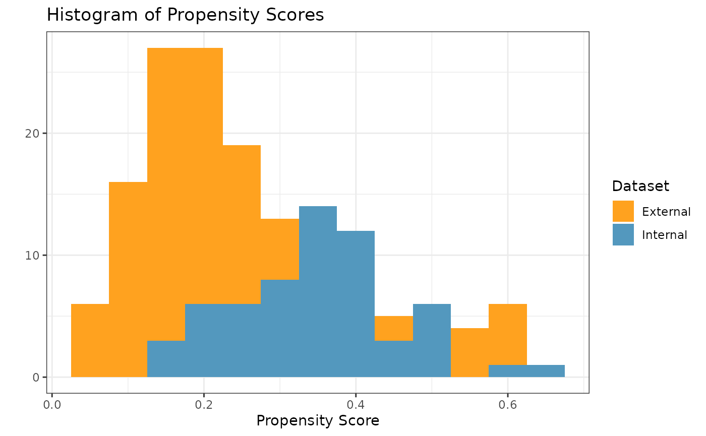

prop_scr_dens(ps_obj, variable = "ipw")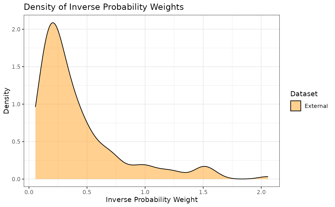

The final plot we might want to look at is a love plot to visualize the absolute standardized mean differences (both unadjusted and adjusted by the IPWs) of the covariates between the internal and external data. To do this, we use the prop_scr_love function. Like the previous function, the only required parameter for this function is the propensity score object, but we can also provide a location along the x-axis for a vertical reference line.

prop_scr_love(ps_obj, reference_line = 0.1)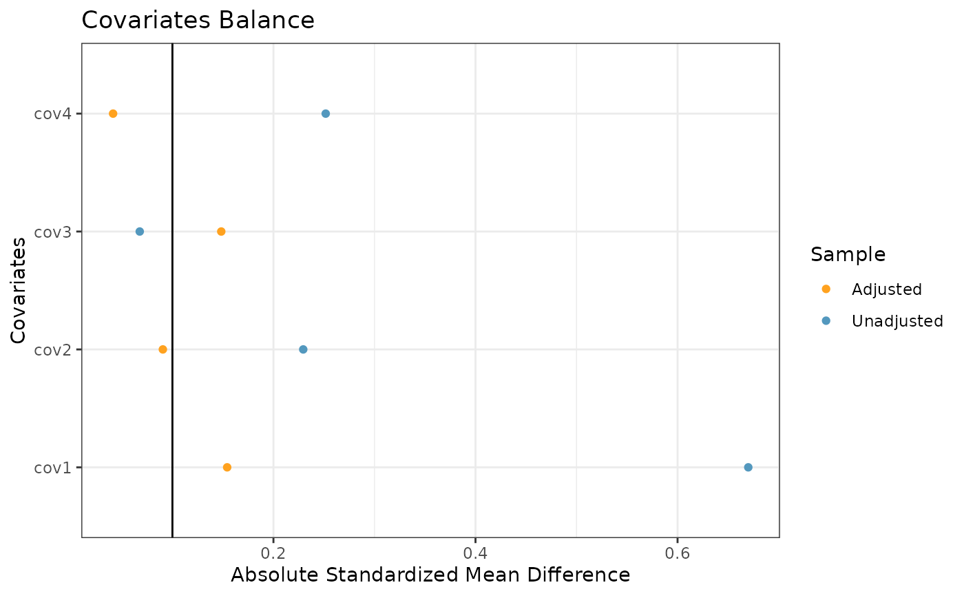

Inverse Probability Weighted Power Prior

Now that we have created and assessed our propensity score object, we can read it into the calc_power_prior_norm function to calculate a normal inverse probability weighted power prior for $\theta_C$ . To calculate the power prior, we need to supply the following information:

weighted object (the propensity score object we created above)
response variable name (in this case $y$ )
initial prior, in the form of a normal distributional object (e.g., $\mbox{N}(0.5, \mbox{sd} = 10)$ )
SD of the external control response data, assumed known

The prior and the external control SD are optional. If no prior is provided, an improper uniform prior will be used for the initial prior; i.e., $\pi(\theta_C) \propto 1$ . If no external control SD or initial prior are specified (i.e., both the prior and external_sd arguments are set as NULL), then a non-standardized $t$ power prior will be created (not covered in this vignette). In this example, we define the initial prior to be a vague normal distribution with a mean 0.5 and SD 10.

Once we have a power prior, we might want to plot it. To do that, we use the plot_dist function.

pwr_prior <- calc_power_prior_norm(ps_obj,
                                   response = y,
                                   prior = dist_normal(0.5, 10), 
                                   external_sd = sd_external_control)
plot_dist(pwr_prior)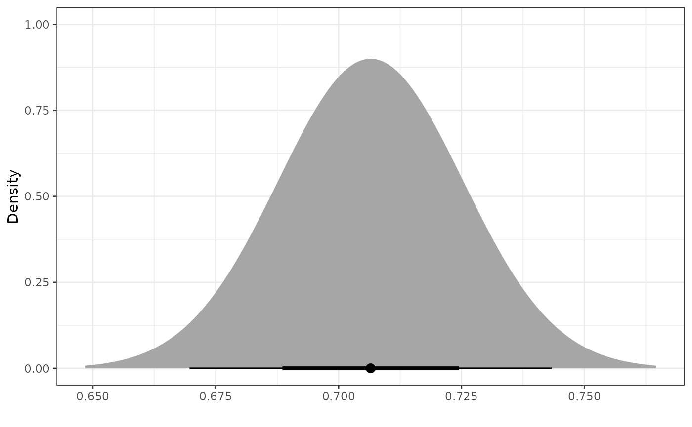

Inverse Probability Weighted Robust Mixture Prior

We can robustify the normal power prior for $\theta_C$ by adding a vague component to create a robust mixture prior (RMP). We define the vague component to be a normal distribution with the same mean as the power prior and a variance that is $n_{ex}$ times greater than the variance of the power prior, where $n_{ex}$ denotes the sample size of the external control arm. To construct the RMP with two components, we use the robustify_norm function and place 0.5 weight on each component. The two components of the resulting RMP are labeled as “informative” and “vague”.

As an alternative to using robustify_norm, we can instead use the dist_mixture function to create a mixture prior with an arbitrary number of normal and/or $t$ components. If any component of the prior is a $t$ distribution, the component will be approximated with the mixture of two normal distributions.

n_external <- nrow(ex_norm_df)
mix_prior <- robustify_norm(pwr_prior, n_external, weights = c(0.5, 0.5))
plot_dist("Power Prior" = pwr_prior,
          "Vague Prior" = dist_normal(mean = mix_means(mix_prior)["vague"],
                                      sd = mix_sigmas(mix_prior)["vague"]),
          "Robust Mixture Prior" = mix_prior)

Posterior Distributions

To create a posterior distribution for $\theta_C$ , we can pass the resulting RMP to the calc_post_norm function. By assuming the SD of the internal response data to be known, the resulting posterior distribution is also a mixture of normal components (the case when the SD is unknown is not covered in this vignette).

Note: when reading internal data directly into calc_post_norm, be sure to include only the arm of interest (e.g., the internal control arm if creating a posterior distribution for $\theta_C$ ).

post_control <- calc_post_norm(filter(int_norm_df, trt == 0),
                               response = y, 
                               prior = mix_prior,
                               internal_sd = sd_internal_control)
plot_dist(post_control)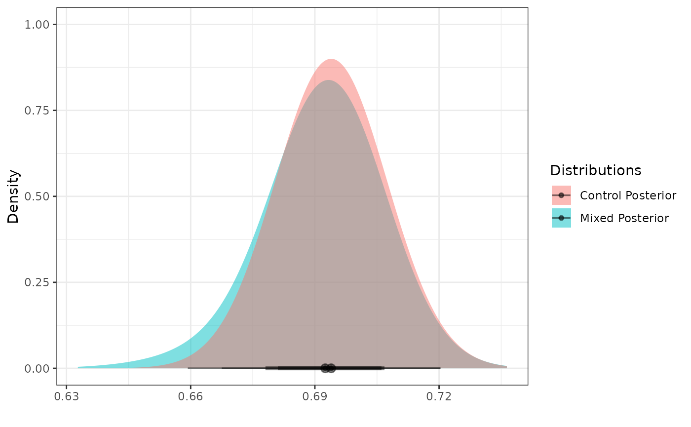

Next, we create a posterior distribution for the mean of the active treatment arm $\theta_T$ by reading the internal data for the corresponding arm into the calc_post_norm function while assuming the SD of the internal active treatment arm to be equal to 0.15. In this case, we use the vague component of the RMP as our normal prior.

As noted earlier, be sure to read in only the data for the internal active treatment arm while excluding the internal control data.

post_treated <- calc_post_norm(internal_data = filter(int_norm_df, trt == 1),
                               response = y,
                               prior = dist_normal(mean = mix_means(mix_prior)["vague"],
                                                   sd = mix_sigmas(mix_prior)["vague"]),
                               internal_sd = sd_internal_treated)
plot_dist("Control Posterior" = post_control,
          "Treatment Posterior" = post_treated)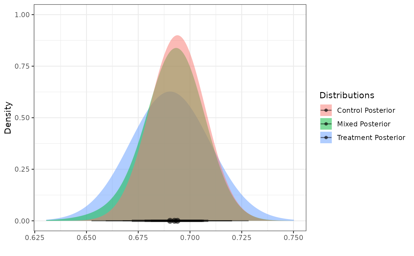

Posterior Summary Statistics and Samples

With our posterior distributions for $\theta_C$ and $\theta_T$ saved as distributional objects, we can use several functions from the distributional package to calculate posterior summary statistics and sample from the distributions. Using the posterior distribution for $\theta_C$ as an example, we illustrate several of these functions below.

Posterior summary statistics:

c(mean = mean(post_control),
  median = median(post_control),
  variance = variance(post_control))
#>        mean      median    variance 
#> 0.675091383 0.675734273 0.000239683

Highest density regions using the hdr function:

hdr(post_control)        # 95% HDR
#> <hdr[1]>
#> [1] [0.6442579, 0.7052676]95
hdr(post_control, 90)    # 90% HDR
#> <hdr[1]>
#> [1] [0.650438, 0.7006585]90

Credible intervals using either the hilo function or the quantile function:

hilo(post_control)       # 95% credible interval
#> <hilo[1]>
#> [1] [0.6420707, 0.7036551]95
hilo(post_control, 90)   # 90% credible interval
#> <hilo[1]>
#> [1] [0.6487183, 0.6992243]90
quantile(post_control, c(.025, .975))[[1]]    # 95% CrI via quantile function
#> [1] 0.6420707 0.7036551

Posterior probabilities (e.g., $Pr(\theta_C < 0.7 | D)$ ) using the cdf function:

cdf(post_control, q = .7)   # Pr(theta_C < 0.7 | D)
#> [1] 0.9554074

Posterior (log) densities at a given value:

density(post_control, at = .7)                # density at 0.7
#> [1] 6.659121
density(post_control, at = .7, log = TRUE)    # log density at 0.7
#> [1] 1.895988

In addition to calculating posterior summary statistics, we can sample from posterior distributions using the generate function. Here, we randomly sample 100,000 draws from the posterior distribution for $\theta_C$ and plot a histogram of the sample.

samp_control <- generate(x = post_control, times = 100000)[[1]]
ggplot(data.frame(samp = samp_control), aes(x = samp)) +
  labs(y = "Density", x = expression(theta[C])) +
  ggtitle(expression(paste("Posterior Samples of ", theta[C]))) +
  geom_histogram(aes(y = after_stat(density)), color = "#5398BE", fill = "#5398BE",
                 position = "identity", binwidth = .01, alpha = 0.5) +
  geom_density(color = "black") +
  theme_bw()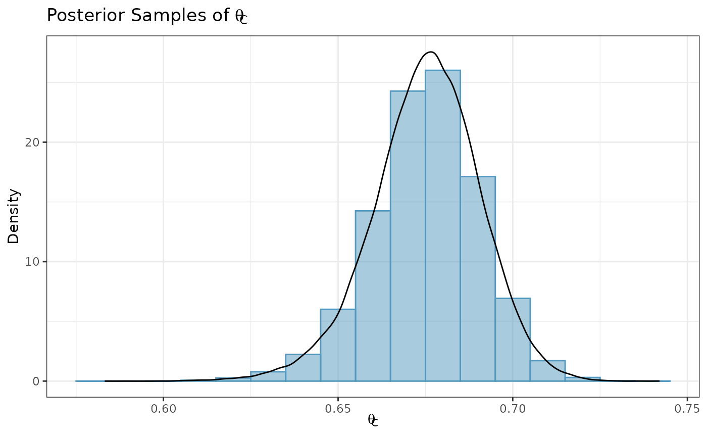

Similarly, we sample from the posterior distribution for $\theta_T$ .

samp_treated <- generate(x = post_treated, times = 100000)[[1]]
ggplot(data.frame(samp = samp_treated), aes(x = samp)) +
  labs(y = "Density", x = expression(theta[T])) +
  ggtitle(expression(paste("Posterior Samples of ", theta[T]))) +
  geom_histogram(aes(y = after_stat(density)), color = "#FFA21F", fill = "#FFA21F",
                 position = "identity", binwidth = .01, alpha = 0.5) +
  geom_density(color = "black") +
  theme_bw()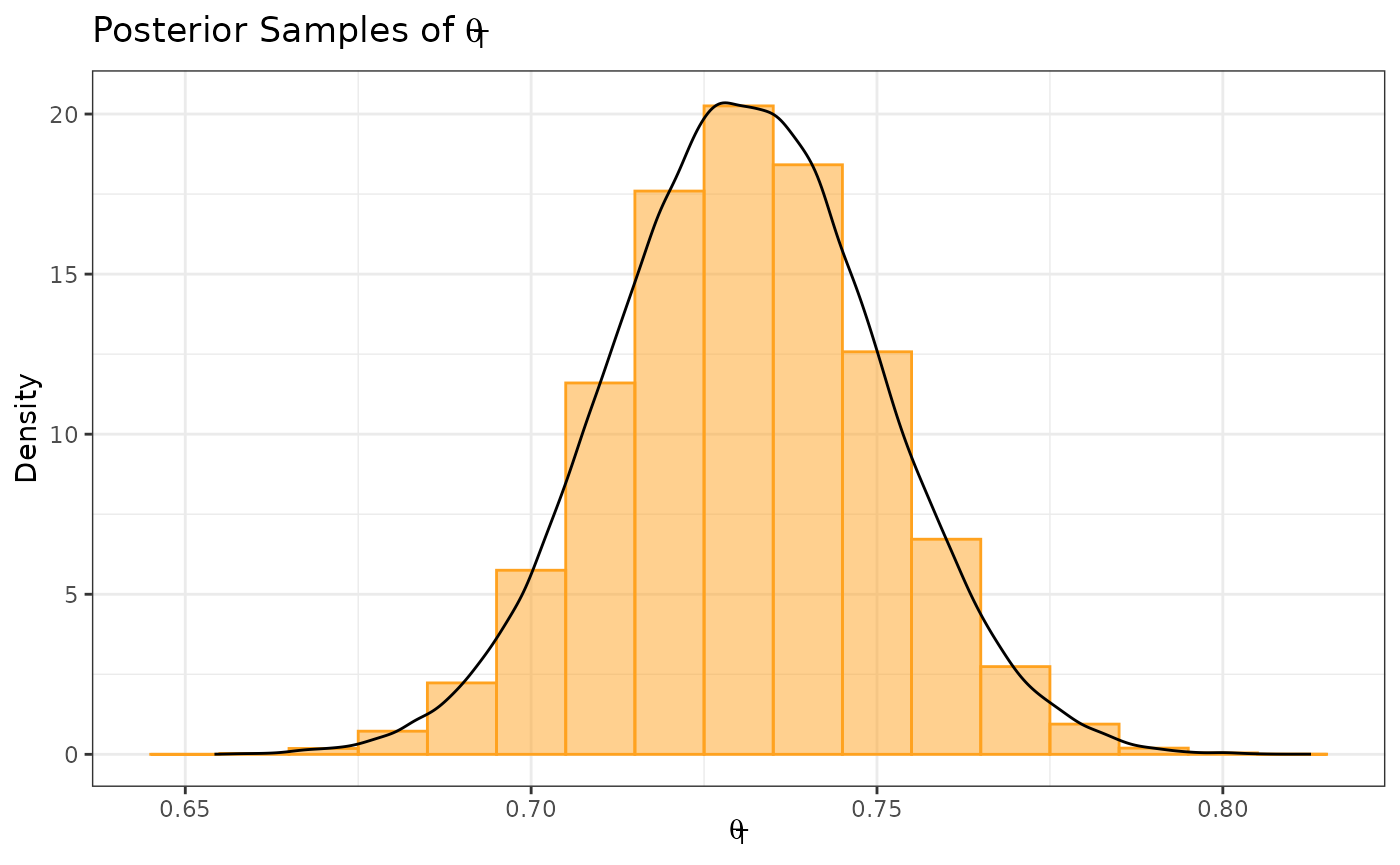

We define our marginal treatment effect to be the difference between the active treatment mean and the control mean (i.e., $\theta_T - \theta_C$ ). We can obtain a sample from the posterior distribution for $\theta_T - \theta_C$ by subtracting the posterior sample of $\theta_C$ from the posterior sample of $\theta_T$ .

samp_trt_diff <- samp_treated - samp_control
ggplot(data.frame(samp = samp_trt_diff), aes(x = samp)) +
  labs(y = "Density", x = expression(paste(theta[T], " - ", theta[C]))) +
  ggtitle(expression(paste("Posterior Samples of ", theta[T], " - ", theta[C]))) +
  geom_histogram(aes(y = after_stat(density)), color = "#FF0000", fill = "#FF0000",
                 position = "identity", binwidth = .01, alpha = 0.5) +
  geom_density(color = "black") +
  theme_bw()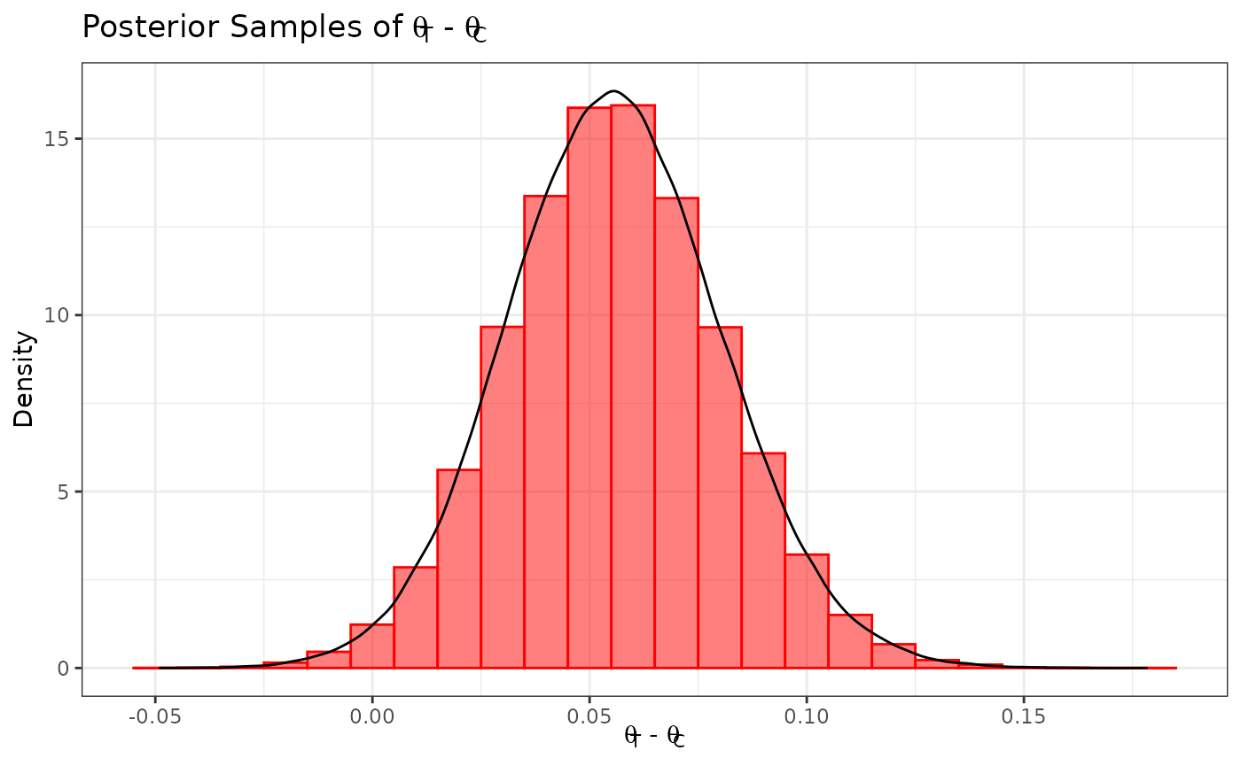

Suppose we want to test the hypotheses $H_0: \theta_T - \theta_C \le 0$ versus $H_1: \theta_T - \theta_C > 0$ . We can use our posterior sample for $\theta_T - \theta_C$ to calculate the posterior probability $Pr(\theta_T - \theta_C > 0 \mid D)$ (i.e., the probability in favor of $H_1$ ), and we conclude that we have sufficient evidence in favor of the alternative hypothesis if $Pr(\theta_T - \theta_C > 0 \mid D) > 0.975$ .

mean(samp_trt_diff > 0)
#> [1] 0.98866

We see that this posterior probability is greater than 0.975, and hence we have sufficient evidence to support the alternative hypothesis.

Using the parameters function from the distributional package, we can extract the parameters of a posterior distribution that consists of a single component (i.e., a single normal distribution). For example, we can extract the mean (mu) and standard deviation (sigma) parameters of the beta posterior distribution for $\theta_T$ .

parameters(post_treated)
#>          mu      sigma
#> 1 0.7307423 0.01929926

For posterior distributions that are a mixture of normal components, we can extract the means and standard deviations of each component using the mix_means and mix_sigmas functions, respectively.

mix_means(post_control)    # means of each normal component
#> informative       vague 
#>   0.6772442   0.6636995
mix_sigmas(post_control)   # SDs of each normal component
#> informative       vague 
#>  0.01361736  0.01929926

We can also use the parameters function to extract the mixture weights associated with the normal components of the posterior distribution for $\theta_C$ .

parameters(post_control)$w[[1]]
#> informative       vague 
#>   0.8410606   0.1589394

Lastly, we calculate the effective sample size of the posterior distribution for $\theta_C$ using the method by Pennello and Thompson (2008). To do so, we first must construct the posterior distribution of $\theta_C$ without borrowing from the external control data (e.g., using a vague prior).

post_control_no_brrw <- calc_post_norm(filter(int_norm_df, trt == 0),
                                       response = y,
                                       prior = dist_normal(mean = mix_means(mix_prior)["vague"],
                                                           sd = mix_sigmas(mix_prior)["vague"]),
                                       internal_sd = sd_internal_control)
n_int_ctrl <- nrow(filter(int_norm_df, trt == 0))   # sample size of internal control arm
var_no_brrw <- variance(post_control_no_brrw)       # post variance of theta_C without borrowing
var_brrw <- variance(post_control)                  # post variance of theta_C with borrowing
ess <- n_int_ctrl * var_no_brrw / var_brrw          # effective sample size
ess
#> [1] 93.23853

References

Psioda, M. A., Bean, N. W., Wright, B. A., Lu, Y., Mantero, A., and Majumdar, A. (2025). Inverse probability weighted Bayesian dynamic borrowing for estimation of marginal treatment effects with application to hybrid control arm oncology studies. Journal of Biopharmaceutical Statistics, 1–23. DOI: 10.1080/10543406.2025.2489285.