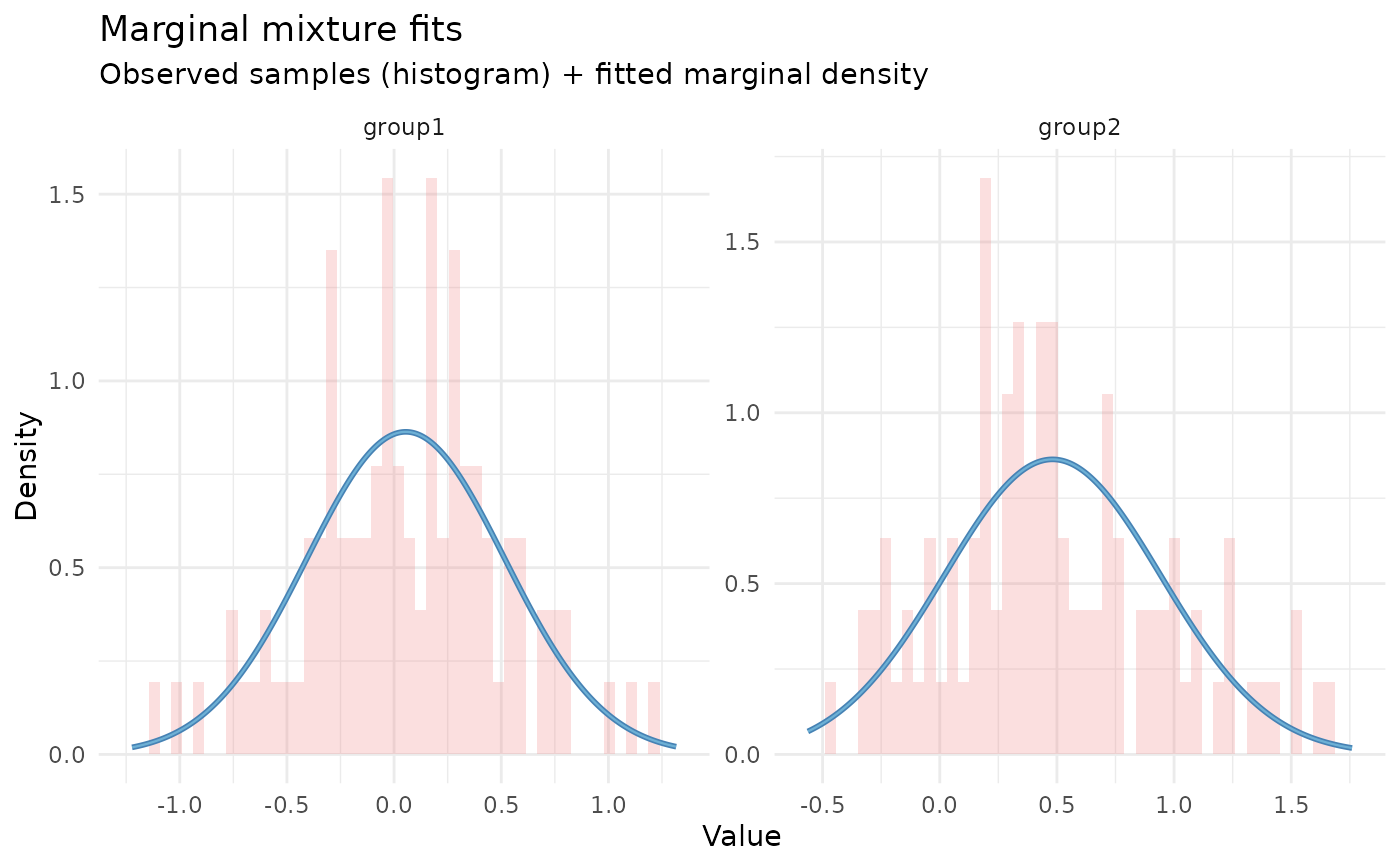
Plot fitted marginal densities or QQ plots for mixture models

Overlays fitted marginal mixture densities from a shrinkr_mixture (returned by fit_mixture()) on top of the observed samples for selected variables, OR creates QQ plots comparing empirical vs fitted quantiles. The function uses the same coercion logic as fit_mixture() (via an internal .coerce_draws_df() helper), ensuring that variable names line up even when users pass a list of matrices.

Important: For multivariate joint fits, this produces marginal overlays (one panel per variable when faceting). Each marginal density is computed by summing the weighted component densities for that variable.

Usage

# S3 method for class 'shrinkr_mixture'
plot(
  x,
  draws = NULL,
  variables = NULL,
  type = c("density", "qq"),
  overlay = c("hist", "kde", "both", "none"),
  bins = 50,
  kde_bw = NULL,
  show_components = TRUE,
  facet = TRUE,
  n_points = 501,
  verbose = FALSE,
  ...
)

Arguments

x: A shrinkr_mixture object from fit_mixture().
draws: Optional samples to show as histogram/KDE or for QQ plot. Accepts any input shape supported by fit_mixture(). When NULL, only fitted curves are drawn (QQ plot requires draws).
variables: Character vector of variables to plot. Defaults to all variables in x$components$variable. Variable names must match the names created by the fitter (and by .coerce_draws_df()).
type: One of c("density","qq"). Default "density" shows density overlay; "qq" creates quantile-quantile plots comparing empirical vs fitted quantiles.
overlay: One of c("hist","kde","both","none"). Default "hist". Only applies when type = "density".
bins: Integer number of bins for the histogram (default 50).
kde_bw: Bandwidth for stats::density(); NULL uses the default. Ignored unless overlay is "kde" or "both".
show_components: Logical; if TRUE (default) overlays per-component curves using component weights, means, and marginal SDs from x$components. Only applies when type = "density".
facet: Logical; if TRUE (default) facet by variable when plotting more than one variable.
n_points: Integer; number of x grid points for evaluating densities (default 501). For QQ plots, this controls the number of quantiles to compare.
verbose: Logical; print brief matching diagnostics.
...: Additional arguments (currently unused).

Value

A ggplot2 object.

Details

Density plots

The total marginal density for each variable $j$ is computed as $$f_j(x)=\sum_{k=1}^{K} w_k \,\phi\!\left(x \mid \mu_{jk},\, \sigma_{jk}\right),$$ using per-component marginal SDs (sd) already stored in x$components.

The plotting range per variable is taken from the sample range if available (with 5% padding), otherwise from mean +/- 4*sd across that variable's components–avoiding non-finite seq() errors when samples are absent.

QQ plots

When type = "qq", the function creates quantile-quantile plots by:

Computing empirical quantiles from the observed data
Computing theoretical quantiles from the fitted mixture CDF via numerical inversion
Plotting empirical vs theoretical quantiles with a 45-degree reference line

Points falling on the reference line indicate good agreement between the fitted mixture and the data. Systematic deviations suggest model misfit.

Examples

set.seed(1)
samples <- list(
  group1 = matrix(rnorm(100, 0.0, 0.5), ncol = 1),
  group2 = matrix(rnorm(100, 0.5, 0.5), ncol = 1)
)
mix <- fit_mixture(samples, K_max = 2, verbose = FALSE)
plot(mix, draws = samples, type = "density", variables = c("group1", "group2"))