Getting Started with shrinkr

What is shrinkr?

shrinkr lets you apply Bayesian hierarchical shrinkage to group-specific estimates in a modular, two-stage workflow:

Stage 1: Fit your model separately for each group (region, hospital, study, etc.) using flat priors
Stage 2: Borrow strength across groups through hierarchical shrinkage

Why use shrinkr?

You’ve already fit separate models and want to pool information afterward
You want modularity to separate model fitting from shrinkage estimation
You want to simplify shrinkage estimation in complex models
You want to try different shrinkage priors without refitting expensive Stage 1 models
You need transparency in how much your results depend on the hierarchical prior
You’re doing meta-analysis or federated learning with summary statistics

library(shrinkr)
library(distributional)
library(posterior)
library(tidyverse)

A Complete Example: Regional Clinical Trial

Imagine a clinical trial run independently in 5 regions. Each region estimated a treatment effect, and now you want to apply shrinkage analysis.

Stage 1: Fit Independent Models with Stan

First, let’s create synthetic trial data:

library(rstan)
set.seed(1104)

true_mu <- 0.5
true_tau <- 0.3
true_effects <- c(0.45, 0.72, 0.38, 0.55, 0.61)

regions <- c("North", "South", "East", "West", "Central")
n_per_region <- c(100, 80, 120, 90, 70)

trial_data <- lapply(seq_along(regions), function(i) {
  n <- n_per_region[i]
  data.frame(
    region = regions[i],
    treatment = rep(c(0, 1), each = n/2),
    outcome = c(
      rnorm(n/2, mean = 0, sd = 1),
      rnorm(n/2, mean = true_effects[i], sd = 1)
    )
  )
}) %>% bind_rows()

head(trial_data)
table(trial_data$region, trial_data$treatment)

#>   region treatment     outcome
#> 1  North         0 -0.04382439
#> 2  North         0  0.64111730
#> 3  North         0 -0.33395868
#> 4  North         0 -2.60279243
#> 5  North         0  1.17838867
#> 6  North         0 -0.20705477
#>          
#>            0  1
#>   Central 35 35
#>   East    60 60
#>   North   50 50
#>   South   40 40
#>   West    45 45

Now we write a Stan model with treatment-by-region interaction:

stan_code <- "
data {
  int<lower=0> N;
  int<lower=1> G;
  vector[N] y;
  vector[N] treatment;
  array[N] int<lower=1,upper=G> region;
}
parameters {
  vector[G] beta_region;
  real<lower=0> sigma;
}
model {
  // IMPORTANT: Flat prior on beta_region - critical for the two-stage approach!
  sigma ~ normal(0, 2);
  for (n in 1:N) {
    y[n] ~ normal(treatment[n] * beta_region[region[n]], sigma);
  }
}
"

regions <- c("North", "South", "East", "West", "Central")
region_indices <- as.integer(factor(trial_data$region, levels = regions))

fit_stan <- stan(
  model_code = stan_code,
  data = list(
    N = nrow(trial_data), G = length(regions),
    y = trial_data$outcome, treatment = trial_data$treatment,
    region = region_indices
  ),
  chains = 4, iter = 2000, warmup = 1000, refresh = 0, seed = 123
)

beta_draws <- rstan::extract(fit_stan, pars = "beta_region")$beta_region
samples_list <- lapply(seq_along(regions), function(i) beta_draws[, i])
names(samples_list) <- regions
samples <- lapply(samples_list, function(x) matrix(x, ncol = 1))

Let’s examine what we got from Stage 1:

stage1_summary <- data.frame(
  region = regions,
  mean   = sapply(samples, mean),
  sd     = sapply(samples, sd),
  lower  = sapply(samples, function(x) quantile(x, 0.025)),
  upper  = sapply(samples, function(x) quantile(x, 0.975))
)

print(stage1_summary)

#>          region      mean        sd      lower     upper
#> North     North 0.6040241 0.1405588 0.33617456 0.8799941
#> South     South 0.6000233 0.1540522 0.29866430 0.8924705
#> East       East 0.6152066 0.1265935 0.36515463 0.8666375
#> West       West 0.7049122 0.1494923 0.41466597 0.9940618
#> Central Central 0.3626256 0.1676080 0.02935275 0.6966270

Stage 1 visualization:

ggplot(stage1_summary, aes(x = region, y = mean)) +
  geom_hline(yintercept = 0, linetype = "dashed", color = "gray50") +
  geom_pointrange(aes(ymin = lower, ymax = upper),
                  size = 0.8, color = "steelblue") +
  labs(
    title    = "Stage 1: Independent Regional Estimates",
    subtitle = "Each region analyzed separately with flat priors",
    x = "Region", y = "Treatment Effect",
    caption = "Points show posterior means; bars show 95% credible intervals"
  ) +
  theme_minimal(base_size = 12)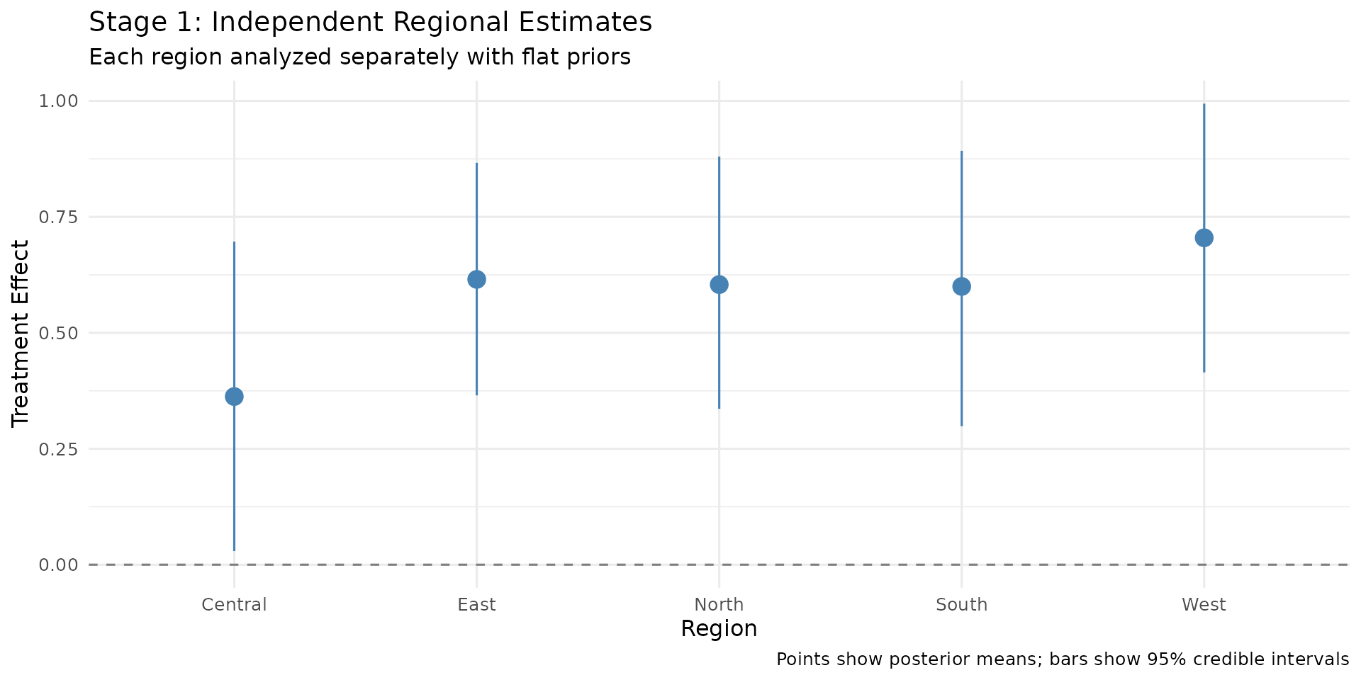

Notice: Central has the widest interval (n=70) and East the narrowest (n=120). Estimates vary considerably — hierarchical shrinkage will borrow strength across regions.

Stage 2: Apply Hierarchical Shrinkage

Step 1: Fit Mixture Approximation

mix <- fit_mixture(samples = samples, K_max = 3, verbose = TRUE)

print(mix)

Check the approximation quality:

# Blue line should overlay the histogram well
plot(mix, draws = samples, type = "density")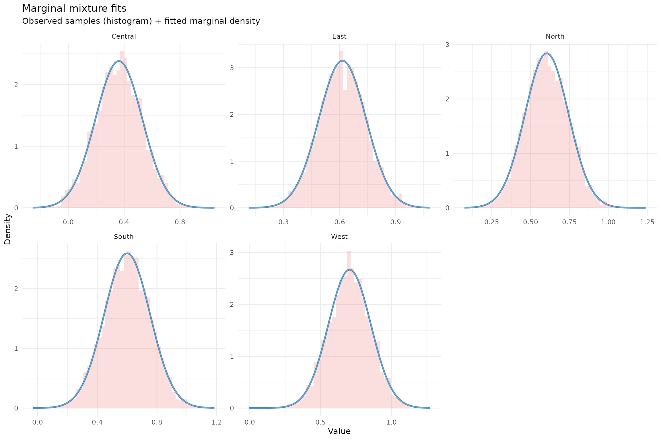


# Points should fall near the diagonal
plot(mix, draws = samples, type = "qq")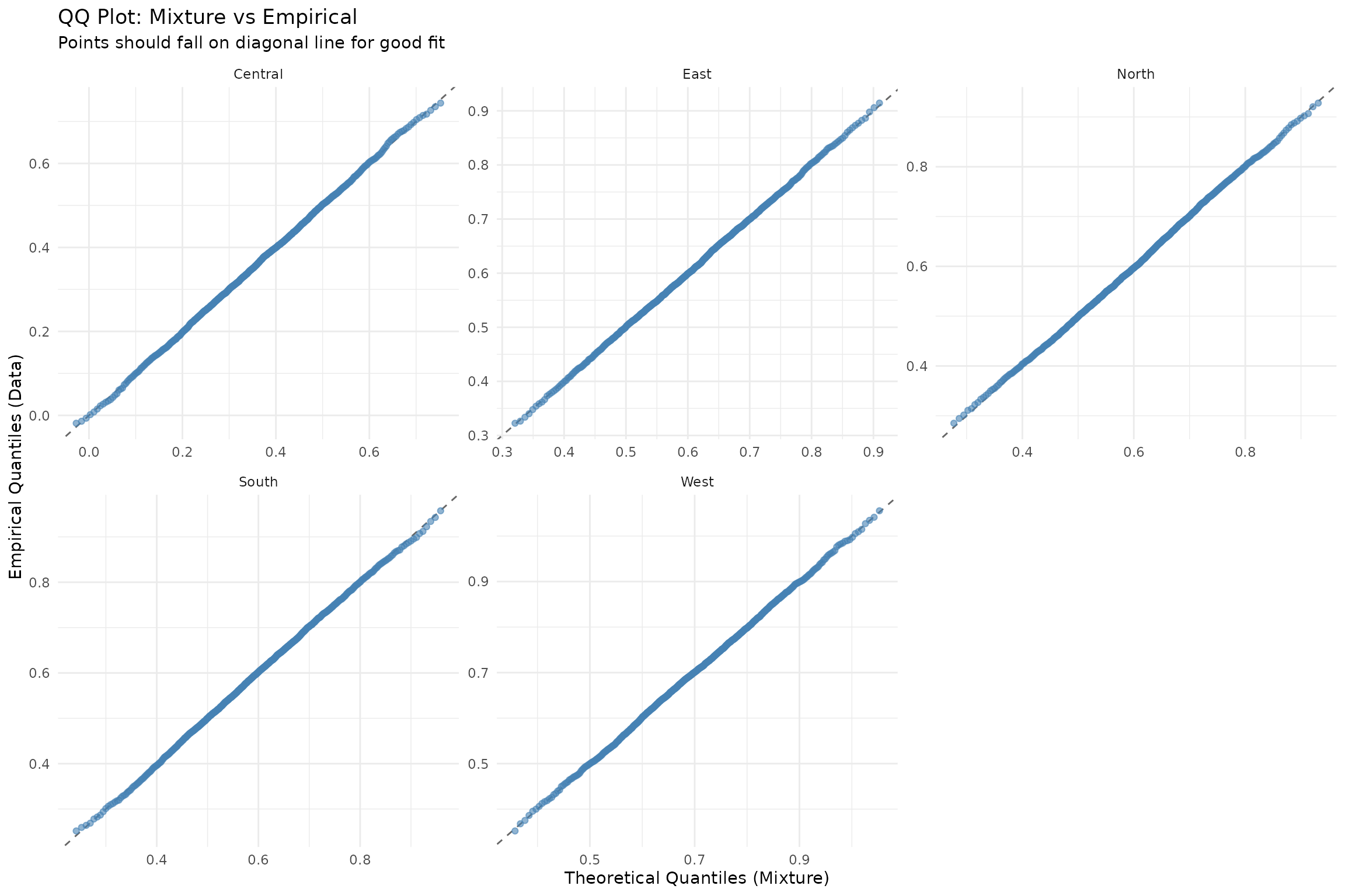

Step 2: Specify Hierarchical Priors

hierarchical_priors <- list(
  mu  = dist_normal(0, 1),
  tau = dist_truncated(dist_student_t(3, 0, 0.5), lower = 0)
)

Check prior implications before fitting:

prior_pred <- sample_prior_predictive(
  hierarchical_priors = hierarchical_priors,
  n_groups = 5,
  n_draws  = 1000
)

cat("Prior on tau (between-region SD):\n")
cat("  Median:", round(median(prior_pred$tau), 2), "\n")
cat("  95% interval:", round(quantile(prior_pred$tau, c(0.025, 0.975)), 2), "\n\n")

cat("Implied variation in regional effects:\n")
cat("  Typical range:", round(median(prior_pred$implied_range), 2), "\n")
cat("  95% interval:", round(quantile(prior_pred$implied_range, c(0.025, 0.975)), 2), "\n")

#> Prior on tau (between-region SD):
#>   Median: 0.38
#>   95% interval: 0.02 1.95
#> Implied variation in regional effects:
#>   Typical range: 0.81
#>   95% interval: 0.03 4.83

plot(prior_pred)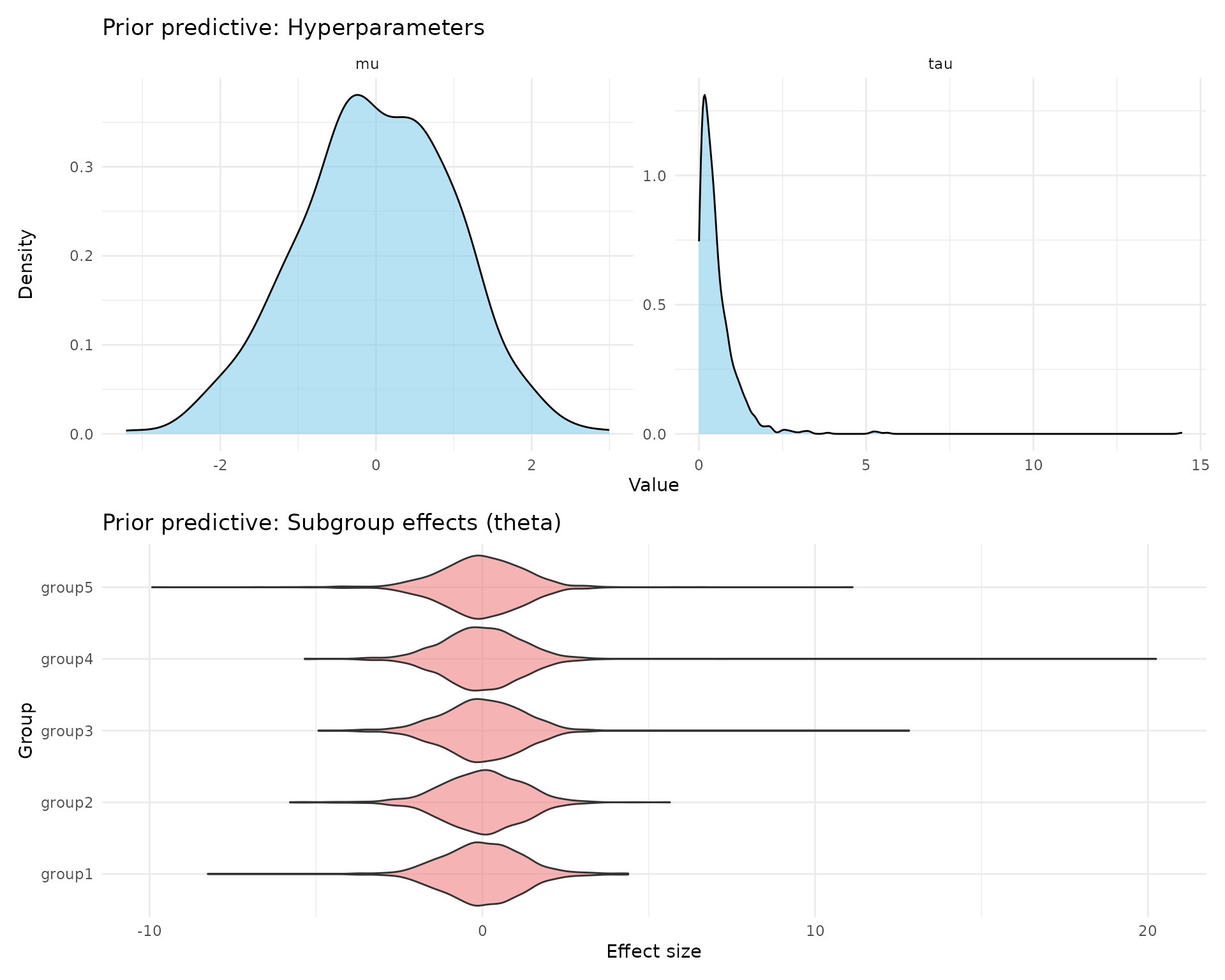

Check what the prior implies about pairwise subgroup differences:

The implied_range above measures max(theta) - min(theta) across all groups for each draw. For a more detailed view, prior_pairwise_differences() computes the distribution of |theta_i - theta_j| for every pair of groups. This is particularly useful for calibrating whether your prior places reasonable probability on clinically meaningful differences.

pw <- prior_pairwise_differences(prior_pred)
print(pw)
#> == Prior Predictive: Pairwise |theta_i - theta_j| ==
#> 
#> Groups:  5 
#> Pairs:   10 
#> Draws:   1000 
#> 
#> Overall quantiles of |theta_i - theta_j|:
#>    q2.5 = 0.005, q25 = 0.094, q50 = 0.302, q75 = 0.752, q97.5 = 2.958 
#> 
#> Per-pair summary:
#> # A tibble: 10 × 6
#>    pair             median    q2.5 q97.5 prob_gt_0.5 prob_gt_1
#>    <chr>             <dbl>   <dbl> <dbl>       <dbl>     <dbl>
#>  1 group1 vs group2  0.314 0.00517  2.94       0.364     0.185
#>  2 group1 vs group3  0.320 0.00507  2.93       0.37      0.182
#>  3 group1 vs group4  0.318 0.00522  3.02       0.362     0.193
#>  4 group1 vs group5  0.298 0.00463  2.95       0.376     0.177
#>  5 group2 vs group3  0.316 0.00555  2.81       0.361     0.185
#>  6 group2 vs group4  0.297 0.00444  2.71       0.35      0.172
#>  7 group2 vs group5  0.297 0.00569  3.07       0.36      0.189
#>  8 group3 vs group4  0.306 0.00333  2.92       0.368     0.167
#>  9 group3 vs group5  0.294 0.00443  3.04       0.336     0.159
#> 10 group4 vs group5  0.277 0.00573  2.90       0.341     0.164
#> 
#> -----------------------------------------------------
#> Use plot() to visualize

# Pooled histogram of |theta_i - theta_j| across all pairs
plot(pw)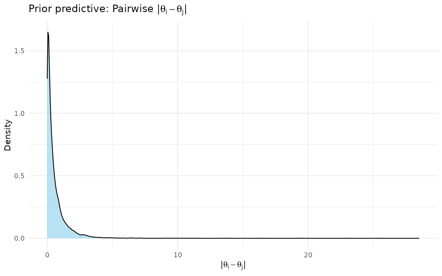

The prob_gt_0.5 and prob_gt_1 columns in the summary show the prior probability of observing pairwise differences exceeding those thresholds — useful for assessing whether your prior is consistent with your clinical expectations about subgroup heterogeneity.

Step 3: Fit the Hierarchical Model

fit <- shrink(
  mixture             = mix,
  hierarchical_priors = hierarchical_priors,
  chains  = 4,
  iter    = 2000,
  warmup  = 1000,
  seed    = 456,
  refresh = 0
)
#> 
#> SAMPLING FOR MODEL 'stage2_shrinkage' NOW (CHAIN 1).
#> Chain 1: 
#> Chain 1: Gradient evaluation took 1.9e-05 seconds
#> Chain 1: 1000 transitions using 10 leapfrog steps per transition would take 0.19 seconds.
#> Chain 1: Adjust your expectations accordingly!
#> Chain 1: 
#> Chain 1: 
#> Chain 1: Iteration:    1 / 2000 [  0%]  (Warmup)
#> Chain 1: Iteration:  100 / 2000 [  5%]  (Warmup)
#> Chain 1: Iteration:  200 / 2000 [ 10%]  (Warmup)
#> Chain 1: Iteration:  300 / 2000 [ 15%]  (Warmup)
#> Chain 1: Iteration:  400 / 2000 [ 20%]  (Warmup)
#> Chain 1: Iteration:  500 / 2000 [ 25%]  (Warmup)
#> Chain 1: Iteration:  600 / 2000 [ 30%]  (Warmup)
#> Chain 1: Iteration:  700 / 2000 [ 35%]  (Warmup)
#> Chain 1: Iteration:  800 / 2000 [ 40%]  (Warmup)
#> Chain 1: Iteration:  900 / 2000 [ 45%]  (Warmup)
#> Chain 1: Iteration: 1000 / 2000 [ 50%]  (Warmup)
#> Chain 1: Iteration: 1001 / 2000 [ 50%]  (Sampling)
#> Chain 1: Iteration: 1100 / 2000 [ 55%]  (Sampling)
#> Chain 1: Iteration: 1200 / 2000 [ 60%]  (Sampling)
#> Chain 1: Iteration: 1300 / 2000 [ 65%]  (Sampling)
#> Chain 1: Iteration: 1400 / 2000 [ 70%]  (Sampling)
#> Chain 1: Iteration: 1500 / 2000 [ 75%]  (Sampling)
#> Chain 1: Iteration: 1600 / 2000 [ 80%]  (Sampling)
#> Chain 1: Iteration: 1700 / 2000 [ 85%]  (Sampling)
#> Chain 1: Iteration: 1800 / 2000 [ 90%]  (Sampling)
#> Chain 1: Iteration: 1900 / 2000 [ 95%]  (Sampling)
#> Chain 1: Iteration: 2000 / 2000 [100%]  (Sampling)
#> Chain 1: 
#> Chain 1:  Elapsed Time: 0.052 seconds (Warm-up)
#> Chain 1:                0.038 seconds (Sampling)
#> Chain 1:                0.09 seconds (Total)
#> Chain 1: 
#> 
#> SAMPLING FOR MODEL 'stage2_shrinkage' NOW (CHAIN 2).
#> Chain 2: 
#> Chain 2: Gradient evaluation took 6e-06 seconds
#> Chain 2: 1000 transitions using 10 leapfrog steps per transition would take 0.06 seconds.
#> Chain 2: Adjust your expectations accordingly!
#> Chain 2: 
#> Chain 2: 
#> Chain 2: Iteration:    1 / 2000 [  0%]  (Warmup)
#> Chain 2: Iteration:  100 / 2000 [  5%]  (Warmup)
#> Chain 2: Iteration:  200 / 2000 [ 10%]  (Warmup)
#> Chain 2: Iteration:  300 / 2000 [ 15%]  (Warmup)
#> Chain 2: Iteration:  400 / 2000 [ 20%]  (Warmup)
#> Chain 2: Iteration:  500 / 2000 [ 25%]  (Warmup)
#> Chain 2: Iteration:  600 / 2000 [ 30%]  (Warmup)
#> Chain 2: Iteration:  700 / 2000 [ 35%]  (Warmup)
#> Chain 2: Iteration:  800 / 2000 [ 40%]  (Warmup)
#> Chain 2: Iteration:  900 / 2000 [ 45%]  (Warmup)
#> Chain 2: Iteration: 1000 / 2000 [ 50%]  (Warmup)
#> Chain 2: Iteration: 1001 / 2000 [ 50%]  (Sampling)
#> Chain 2: Iteration: 1100 / 2000 [ 55%]  (Sampling)
#> Chain 2: Iteration: 1200 / 2000 [ 60%]  (Sampling)
#> Chain 2: Iteration: 1300 / 2000 [ 65%]  (Sampling)
#> Chain 2: Iteration: 1400 / 2000 [ 70%]  (Sampling)
#> Chain 2: Iteration: 1500 / 2000 [ 75%]  (Sampling)
#> Chain 2: Iteration: 1600 / 2000 [ 80%]  (Sampling)
#> Chain 2: Iteration: 1700 / 2000 [ 85%]  (Sampling)
#> Chain 2: Iteration: 1800 / 2000 [ 90%]  (Sampling)
#> Chain 2: Iteration: 1900 / 2000 [ 95%]  (Sampling)
#> Chain 2: Iteration: 2000 / 2000 [100%]  (Sampling)
#> Chain 2: 
#> Chain 2:  Elapsed Time: 0.051 seconds (Warm-up)
#> Chain 2:                0.029 seconds (Sampling)
#> Chain 2:                0.08 seconds (Total)
#> Chain 2: 
#> 
#> SAMPLING FOR MODEL 'stage2_shrinkage' NOW (CHAIN 3).
#> Chain 3: 
#> Chain 3: Gradient evaluation took 6e-06 seconds
#> Chain 3: 1000 transitions using 10 leapfrog steps per transition would take 0.06 seconds.
#> Chain 3: Adjust your expectations accordingly!
#> Chain 3: 
#> Chain 3: 
#> Chain 3: Iteration:    1 / 2000 [  0%]  (Warmup)
#> Chain 3: Iteration:  100 / 2000 [  5%]  (Warmup)
#> Chain 3: Iteration:  200 / 2000 [ 10%]  (Warmup)
#> Chain 3: Iteration:  300 / 2000 [ 15%]  (Warmup)
#> Chain 3: Iteration:  400 / 2000 [ 20%]  (Warmup)
#> Chain 3: Iteration:  500 / 2000 [ 25%]  (Warmup)
#> Chain 3: Iteration:  600 / 2000 [ 30%]  (Warmup)
#> Chain 3: Iteration:  700 / 2000 [ 35%]  (Warmup)
#> Chain 3: Iteration:  800 / 2000 [ 40%]  (Warmup)
#> Chain 3: Iteration:  900 / 2000 [ 45%]  (Warmup)
#> Chain 3: Iteration: 1000 / 2000 [ 50%]  (Warmup)
#> Chain 3: Iteration: 1001 / 2000 [ 50%]  (Sampling)
#> Chain 3: Iteration: 1100 / 2000 [ 55%]  (Sampling)
#> Chain 3: Iteration: 1200 / 2000 [ 60%]  (Sampling)
#> Chain 3: Iteration: 1300 / 2000 [ 65%]  (Sampling)
#> Chain 3: Iteration: 1400 / 2000 [ 70%]  (Sampling)
#> Chain 3: Iteration: 1500 / 2000 [ 75%]  (Sampling)
#> Chain 3: Iteration: 1600 / 2000 [ 80%]  (Sampling)
#> Chain 3: Iteration: 1700 / 2000 [ 85%]  (Sampling)
#> Chain 3: Iteration: 1800 / 2000 [ 90%]  (Sampling)
#> Chain 3: Iteration: 1900 / 2000 [ 95%]  (Sampling)
#> Chain 3: Iteration: 2000 / 2000 [100%]  (Sampling)
#> Chain 3: 
#> Chain 3:  Elapsed Time: 0.052 seconds (Warm-up)
#> Chain 3:                0.032 seconds (Sampling)
#> Chain 3:                0.084 seconds (Total)
#> Chain 3: 
#> 
#> SAMPLING FOR MODEL 'stage2_shrinkage' NOW (CHAIN 4).
#> Chain 4: 
#> Chain 4: Gradient evaluation took 6e-06 seconds
#> Chain 4: 1000 transitions using 10 leapfrog steps per transition would take 0.06 seconds.
#> Chain 4: Adjust your expectations accordingly!
#> Chain 4: 
#> Chain 4: 
#> Chain 4: Iteration:    1 / 2000 [  0%]  (Warmup)
#> Chain 4: Iteration:  100 / 2000 [  5%]  (Warmup)
#> Chain 4: Iteration:  200 / 2000 [ 10%]  (Warmup)
#> Chain 4: Iteration:  300 / 2000 [ 15%]  (Warmup)
#> Chain 4: Iteration:  400 / 2000 [ 20%]  (Warmup)
#> Chain 4: Iteration:  500 / 2000 [ 25%]  (Warmup)
#> Chain 4: Iteration:  600 / 2000 [ 30%]  (Warmup)
#> Chain 4: Iteration:  700 / 2000 [ 35%]  (Warmup)
#> Chain 4: Iteration:  800 / 2000 [ 40%]  (Warmup)
#> Chain 4: Iteration:  900 / 2000 [ 45%]  (Warmup)
#> Chain 4: Iteration: 1000 / 2000 [ 50%]  (Warmup)
#> Chain 4: Iteration: 1001 / 2000 [ 50%]  (Sampling)
#> Chain 4: Iteration: 1100 / 2000 [ 55%]  (Sampling)
#> Chain 4: Iteration: 1200 / 2000 [ 60%]  (Sampling)
#> Chain 4: Iteration: 1300 / 2000 [ 65%]  (Sampling)
#> Chain 4: Iteration: 1400 / 2000 [ 70%]  (Sampling)
#> Chain 4: Iteration: 1500 / 2000 [ 75%]  (Sampling)
#> Chain 4: Iteration: 1600 / 2000 [ 80%]  (Sampling)
#> Chain 4: Iteration: 1700 / 2000 [ 85%]  (Sampling)
#> Chain 4: Iteration: 1800 / 2000 [ 90%]  (Sampling)
#> Chain 4: Iteration: 1900 / 2000 [ 95%]  (Sampling)
#> Chain 4: Iteration: 2000 / 2000 [100%]  (Sampling)
#> Chain 4: 
#> Chain 4:  Elapsed Time: 0.048 seconds (Warm-up)
#> Chain 4:                0.041 seconds (Sampling)
#> Chain 4:                0.089 seconds (Total)
#> Chain 4:

print(fit)
#> # A tibble: 3 × 7
#>   variable      mean     sd      q2.5     q50 q97.5  rhat
#>   <chr>        <dbl>  <dbl>     <dbl>   <dbl> <dbl> <dbl>
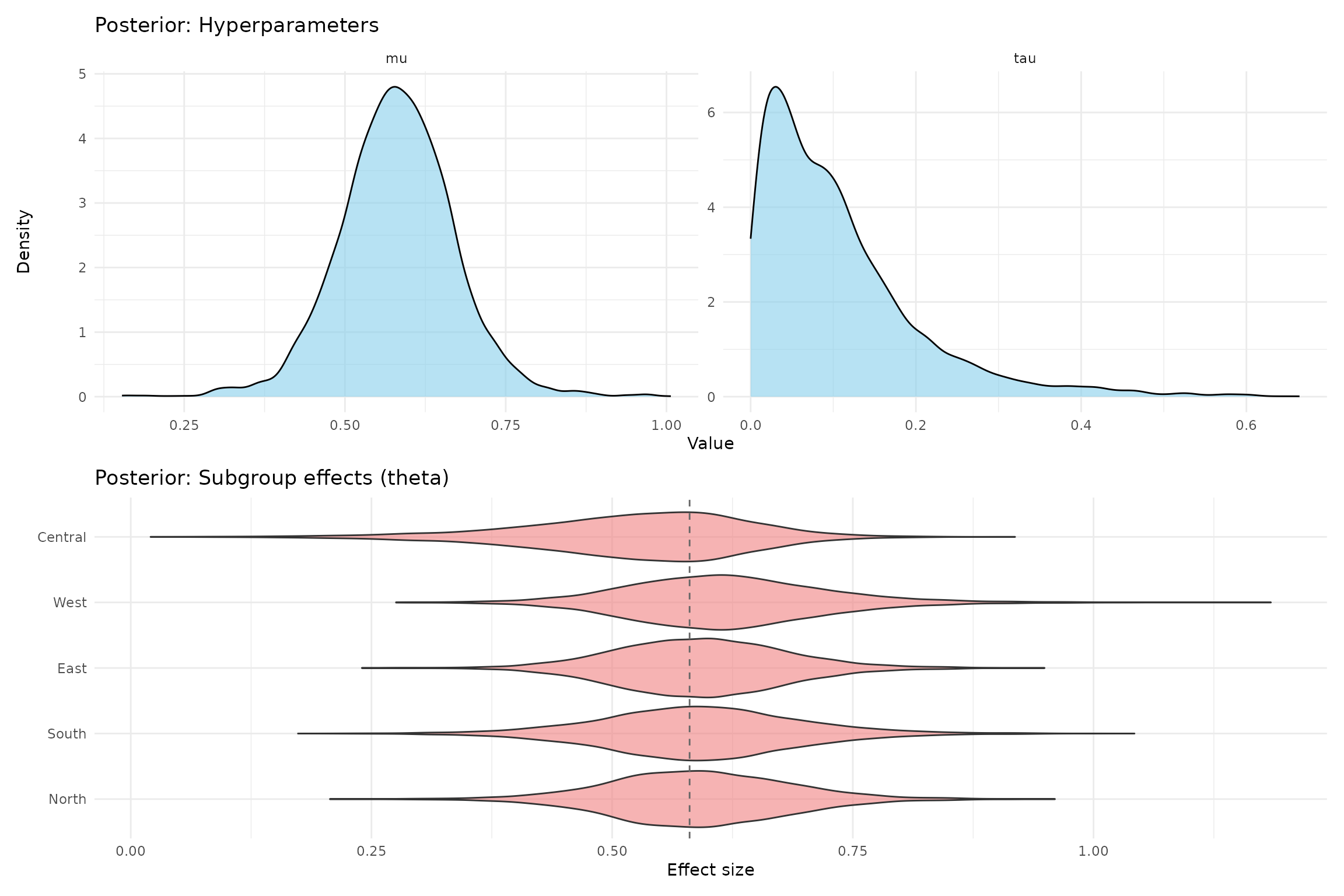
#> 1 mu          0.580  0.0901 0.408     0.580   0.759  1.00
#> 2 tau         0.106  0.0962 0.00407   0.0833  0.382  1.00
#> 3 tau_squared 0.0206 0.0405 0.0000166 0.00694 0.146  1.00

Step 4: Examine Results

mu_tau <- extract_mu_tau(fit)

cat("Overall treatment effect (mu):\n")
#> Overall treatment effect (mu):
cat("  Mean:", round(mean(mu_tau$mu), 3), "\n")
#>   Mean: 0.58
cat("  95% CI:", round(quantile(mu_tau$mu, c(0.025, 0.975)), 3), "\n\n")
#>   95% CI: 0.408 0.759

cat("Between-region heterogeneity (tau):\n")
#> Between-region heterogeneity (tau):
cat("  Mean:", round(mean(mu_tau$tau), 3), "\n")
#>   Mean: 0.106
cat("  95% CI:", round(quantile(mu_tau$tau, c(0.025, 0.975)), 3), "\n")
#>   95% CI: 0.004 0.382

theta_summary <- summarize_theta(fit)
print(theta_summary)
#> # A tibble: 5 × 9
#>   group    mean     sd  q2.5   q50 q97.5  rhat ess_bulk ess_tail
#>   <chr>   <dbl>  <dbl> <dbl> <dbl> <dbl> <dbl>    <dbl>    <dbl>
#> 1 North   0.589 0.0949 0.406 0.588 0.779  1.00    4705.    3346.
#> 2 South   0.590 0.104  0.384 0.589 0.802  1.00    4419.    2962.
#> 3 East    0.592 0.0895 0.421 0.591 0.776  1.00    5150.    3358.
#> 4 West    0.617 0.103  0.428 0.612 0.840  1.00    3966.    3053.
#> 5 Central 0.524 0.117  0.256 0.537 0.721  1.00    2609.    2684.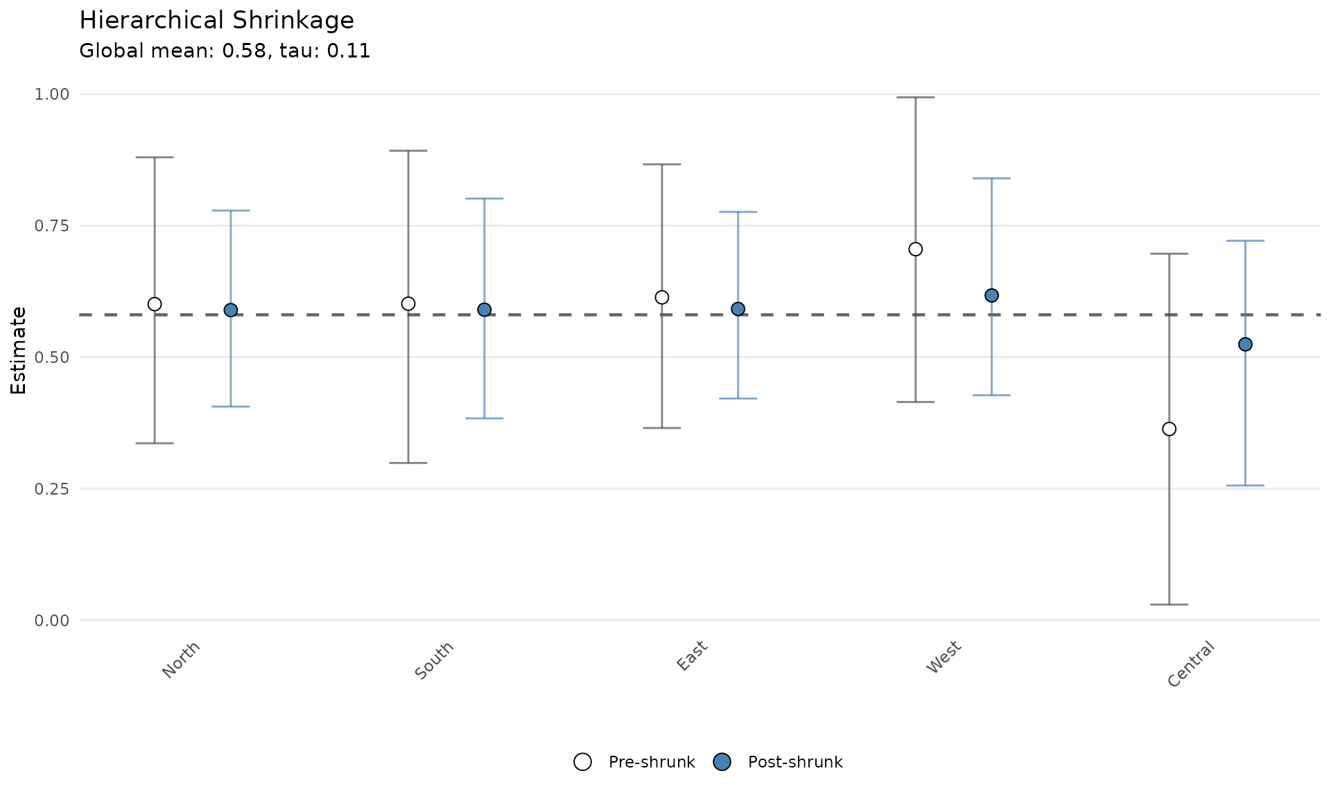

Step 5: Visualize Shrinkage

plot(fit)

Key observations:

Central (most uncertain) shrinks most toward the mean
East (most precise) shrinks least
This is adaptive shrinkage: uncertain estimates borrow more

plot(fit, type = "diagnostics")

Alternative Input: Using Summary Statistics Only

If you only have published means and standard errors (no full posteriors), you can use the MLE approach:

mle_estimates <- sapply(samples, mean)
mle_variances <- sapply(samples, var)

fit_mle <- shrink(
  mle                 = mle_estimates,
  var_matrix          = mle_variances,
  hierarchical_priors = hierarchical_priors,
  chains  = 4,
  iter    = 2000,
  warmup  = 1000,
  seed    = 456,
  refresh = 0
)
#> 
#> SAMPLING FOR MODEL 'stage2_shrinkage' NOW (CHAIN 1).
#> Chain 1: 
#> Chain 1: Gradient evaluation took 1.2e-05 seconds
#> Chain 1: 1000 transitions using 10 leapfrog steps per transition would take 0.12 seconds.
#> Chain 1: Adjust your expectations accordingly!
#> Chain 1: 
#> Chain 1: 
#> Chain 1: Iteration:    1 / 2000 [  0%]  (Warmup)
#> Chain 1: Iteration:  100 / 2000 [  5%]  (Warmup)
#> Chain 1: Iteration:  200 / 2000 [ 10%]  (Warmup)
#> Chain 1: Iteration:  300 / 2000 [ 15%]  (Warmup)
#> Chain 1: Iteration:  400 / 2000 [ 20%]  (Warmup)
#> Chain 1: Iteration:  500 / 2000 [ 25%]  (Warmup)
#> Chain 1: Iteration:  600 / 2000 [ 30%]  (Warmup)
#> Chain 1: Iteration:  700 / 2000 [ 35%]  (Warmup)
#> Chain 1: Iteration:  800 / 2000 [ 40%]  (Warmup)
#> Chain 1: Iteration:  900 / 2000 [ 45%]  (Warmup)
#> Chain 1: Iteration: 1000 / 2000 [ 50%]  (Warmup)
#> Chain 1: Iteration: 1001 / 2000 [ 50%]  (Sampling)
#> Chain 1: Iteration: 1100 / 2000 [ 55%]  (Sampling)
#> Chain 1: Iteration: 1200 / 2000 [ 60%]  (Sampling)
#> Chain 1: Iteration: 1300 / 2000 [ 65%]  (Sampling)
#> Chain 1: Iteration: 1400 / 2000 [ 70%]  (Sampling)
#> Chain 1: Iteration: 1500 / 2000 [ 75%]  (Sampling)
#> Chain 1: Iteration: 1600 / 2000 [ 80%]  (Sampling)
#> Chain 1: Iteration: 1700 / 2000 [ 85%]  (Sampling)
#> Chain 1: Iteration: 1800 / 2000 [ 90%]  (Sampling)
#> Chain 1: Iteration: 1900 / 2000 [ 95%]  (Sampling)
#> Chain 1: Iteration: 2000 / 2000 [100%]  (Sampling)
#> Chain 1: 
#> Chain 1:  Elapsed Time: 0.052 seconds (Warm-up)
#> Chain 1:                0.036 seconds (Sampling)
#> Chain 1:                0.088 seconds (Total)
#> Chain 1: 
#> 
#> SAMPLING FOR MODEL 'stage2_shrinkage' NOW (CHAIN 2).
#> Chain 2: 
#> Chain 2: Gradient evaluation took 7e-06 seconds
#> Chain 2: 1000 transitions using 10 leapfrog steps per transition would take 0.07 seconds.
#> Chain 2: Adjust your expectations accordingly!
#> Chain 2: 
#> Chain 2: 
#> Chain 2: Iteration:    1 / 2000 [  0%]  (Warmup)
#> Chain 2: Iteration:  100 / 2000 [  5%]  (Warmup)
#> Chain 2: Iteration:  200 / 2000 [ 10%]  (Warmup)
#> Chain 2: Iteration:  300 / 2000 [ 15%]  (Warmup)
#> Chain 2: Iteration:  400 / 2000 [ 20%]  (Warmup)
#> Chain 2: Iteration:  500 / 2000 [ 25%]  (Warmup)
#> Chain 2: Iteration:  600 / 2000 [ 30%]  (Warmup)
#> Chain 2: Iteration:  700 / 2000 [ 35%]  (Warmup)
#> Chain 2: Iteration:  800 / 2000 [ 40%]  (Warmup)
#> Chain 2: Iteration:  900 / 2000 [ 45%]  (Warmup)
#> Chain 2: Iteration: 1000 / 2000 [ 50%]  (Warmup)
#> Chain 2: Iteration: 1001 / 2000 [ 50%]  (Sampling)
#> Chain 2: Iteration: 1100 / 2000 [ 55%]  (Sampling)
#> Chain 2: Iteration: 1200 / 2000 [ 60%]  (Sampling)
#> Chain 2: Iteration: 1300 / 2000 [ 65%]  (Sampling)
#> Chain 2: Iteration: 1400 / 2000 [ 70%]  (Sampling)
#> Chain 2: Iteration: 1500 / 2000 [ 75%]  (Sampling)
#> Chain 2: Iteration: 1600 / 2000 [ 80%]  (Sampling)
#> Chain 2: Iteration: 1700 / 2000 [ 85%]  (Sampling)
#> Chain 2: Iteration: 1800 / 2000 [ 90%]  (Sampling)
#> Chain 2: Iteration: 1900 / 2000 [ 95%]  (Sampling)
#> Chain 2: Iteration: 2000 / 2000 [100%]  (Sampling)
#> Chain 2: 
#> Chain 2:  Elapsed Time: 0.05 seconds (Warm-up)
#> Chain 2:                0.04 seconds (Sampling)
#> Chain 2:                0.09 seconds (Total)
#> Chain 2: 
#> 
#> SAMPLING FOR MODEL 'stage2_shrinkage' NOW (CHAIN 3).
#> Chain 3: 
#> Chain 3: Gradient evaluation took 6e-06 seconds
#> Chain 3: 1000 transitions using 10 leapfrog steps per transition would take 0.06 seconds.
#> Chain 3: Adjust your expectations accordingly!
#> Chain 3: 
#> Chain 3: 
#> Chain 3: Iteration:    1 / 2000 [  0%]  (Warmup)
#> Chain 3: Iteration:  100 / 2000 [  5%]  (Warmup)
#> Chain 3: Iteration:  200 / 2000 [ 10%]  (Warmup)
#> Chain 3: Iteration:  300 / 2000 [ 15%]  (Warmup)
#> Chain 3: Iteration:  400 / 2000 [ 20%]  (Warmup)
#> Chain 3: Iteration:  500 / 2000 [ 25%]  (Warmup)
#> Chain 3: Iteration:  600 / 2000 [ 30%]  (Warmup)
#> Chain 3: Iteration:  700 / 2000 [ 35%]  (Warmup)
#> Chain 3: Iteration:  800 / 2000 [ 40%]  (Warmup)
#> Chain 3: Iteration:  900 / 2000 [ 45%]  (Warmup)
#> Chain 3: Iteration: 1000 / 2000 [ 50%]  (Warmup)
#> Chain 3: Iteration: 1001 / 2000 [ 50%]  (Sampling)
#> Chain 3: Iteration: 1100 / 2000 [ 55%]  (Sampling)
#> Chain 3: Iteration: 1200 / 2000 [ 60%]  (Sampling)
#> Chain 3: Iteration: 1300 / 2000 [ 65%]  (Sampling)
#> Chain 3: Iteration: 1400 / 2000 [ 70%]  (Sampling)
#> Chain 3: Iteration: 1500 / 2000 [ 75%]  (Sampling)
#> Chain 3: Iteration: 1600 / 2000 [ 80%]  (Sampling)
#> Chain 3: Iteration: 1700 / 2000 [ 85%]  (Sampling)
#> Chain 3: Iteration: 1800 / 2000 [ 90%]  (Sampling)
#> Chain 3: Iteration: 1900 / 2000 [ 95%]  (Sampling)
#> Chain 3: Iteration: 2000 / 2000 [100%]  (Sampling)
#> Chain 3: 
#> Chain 3:  Elapsed Time: 0.047 seconds (Warm-up)
#> Chain 3:                0.04 seconds (Sampling)
#> Chain 3:                0.087 seconds (Total)
#> Chain 3: 
#> 
#> SAMPLING FOR MODEL 'stage2_shrinkage' NOW (CHAIN 4).
#> Chain 4: 
#> Chain 4: Gradient evaluation took 6e-06 seconds
#> Chain 4: 1000 transitions using 10 leapfrog steps per transition would take 0.06 seconds.
#> Chain 4: Adjust your expectations accordingly!
#> Chain 4: 
#> Chain 4: 
#> Chain 4: Iteration:    1 / 2000 [  0%]  (Warmup)
#> Chain 4: Iteration:  100 / 2000 [  5%]  (Warmup)
#> Chain 4: Iteration:  200 / 2000 [ 10%]  (Warmup)
#> Chain 4: Iteration:  300 / 2000 [ 15%]  (Warmup)
#> Chain 4: Iteration:  400 / 2000 [ 20%]  (Warmup)
#> Chain 4: Iteration:  500 / 2000 [ 25%]  (Warmup)
#> Chain 4: Iteration:  600 / 2000 [ 30%]  (Warmup)
#> Chain 4: Iteration:  700 / 2000 [ 35%]  (Warmup)
#> Chain 4: Iteration:  800 / 2000 [ 40%]  (Warmup)
#> Chain 4: Iteration:  900 / 2000 [ 45%]  (Warmup)
#> Chain 4: Iteration: 1000 / 2000 [ 50%]  (Warmup)
#> Chain 4: Iteration: 1001 / 2000 [ 50%]  (Sampling)
#> Chain 4: Iteration: 1100 / 2000 [ 55%]  (Sampling)
#> Chain 4: Iteration: 1200 / 2000 [ 60%]  (Sampling)
#> Chain 4: Iteration: 1300 / 2000 [ 65%]  (Sampling)
#> Chain 4: Iteration: 1400 / 2000 [ 70%]  (Sampling)
#> Chain 4: Iteration: 1500 / 2000 [ 75%]  (Sampling)
#> Chain 4: Iteration: 1600 / 2000 [ 80%]  (Sampling)
#> Chain 4: Iteration: 1700 / 2000 [ 85%]  (Sampling)
#> Chain 4: Iteration: 1800 / 2000 [ 90%]  (Sampling)
#> Chain 4: Iteration: 1900 / 2000 [ 95%]  (Sampling)
#> Chain 4: Iteration: 2000 / 2000 [100%]  (Sampling)
#> Chain 4: 
#> Chain 4:  Elapsed Time: 0.049 seconds (Warm-up)
#> Chain 4:                0.033 seconds (Sampling)
#> Chain 4:                0.082 seconds (Total)
#> Chain 4:

mu_tau_mle <- extract_mu_tau(fit_mle)

cat("Mixture approach:\n")
#> Mixture approach:
cat("  mu =",  round(mean(mu_tau$mu), 3), "\n")
#>   mu = 0.58
cat("  tau =", round(mean(mu_tau$tau), 3), "\n\n")
#>   tau = 0.106

cat("MLE approach:\n")
#> MLE approach:
cat("  mu =",  round(mean(mu_tau_mle$mu), 3), "\n")
#>   mu = 0.584
cat("  tau =", round(mean(mu_tau_mle$tau), 3), "\n")
#>   tau = 0.113

Method	Use When	Pros	Cons
Mixture	You have full posteriors	Captures non-normality; More accurate	Requires posterior samples
MLE	Only means + SEs available	Simpler; Works with published data	Assumes normality

Complete Stan → shrinkr Workflow Summary

# 1. Write Stan model with FLAT PRIORS on parameters of interest
stan_code <- "
data {
  int<lower=0> N;
  int<lower=1> G;
  vector[N] y;
  vector[N] treatment;
  array[N] int<lower=1,upper=G> group;
}
parameters {
  vector[G] theta;  // Group-specific effects - NO PRIOR SPECIFIED
  real<lower=0> sigma;
}
model {
  sigma ~ normal(0, 2);
  for (n in 1:N) {
    y[n] ~ normal(treatment[n] * theta[group[n]], sigma);
  }
}
"

# 2. Fit model once to get all group effects, extract posteriors
group_indices <- as.integer(factor(data$group, levels = groups))
fit_stan <- stan(
  model_code = stan_code,
  data = list(N = nrow(data), G = length(groups),
              y = data$y, treatment = data$treatment,
              group = group_indices),
  chains = 4, iter = 2000, warmup = 1000, refresh = 0
)

theta_draws <- extract(fit_stan)$theta
samples <- lapply(seq_along(groups), function(i) matrix(theta_draws[, i], ncol = 1))
names(samples) <- groups

# 3. Fit mixture approximation and check quality
mix <- fit_mixture(samples, K_max = 3)
plot(mix, draws = samples)

# 4. Specify and check hierarchical priors
priors <- list(
  mu  = dist_normal(0, 5),
  tau = dist_truncated(dist_student_t(3, 0, 1), lower = 0)
)
plot(sample_prior_predictive(priors, n_groups = length(groups)))

# 5. Fit, extract, and visualize
fit <- shrink(mixture = mix, hierarchical_priors = priors)
plot(fit)
summarize_theta(fit)
extract_mu_tau(fit)

Key Concepts Checklist

Stage 1 uses flat priors - This is critical! Don’t specify a prior on the parameter you’ll shrink
Mixture approximation - Allows shrinkr to work with any posterior shape; check quality with plot()
Hierarchical priors - Applied only in Stage 2; use sample_prior_predictive() to understand implications
Adaptive shrinkage - Uncertain estimates borrow more; precise estimates borrow less
Diagnostics matter - Always check mixture fit, prior-data agreement, and MCMC convergence

Common Pitfalls to Avoid

Using informative priors in Stage 1 - This creates “double priors” and breaks the equivalence
Skipping mixture quality checks - Poor approximation → biased shrinkage, run: plot(mix, draws = samples)
Ignoring prior implications - Your prior might be too strong or weak, run: sample_prior_predictive() and plot()
Not checking convergence - MCMC diagnostics apply to Stage 2 too, check: fit$diagnostics, Rhat, ESS

Next Steps

Advanced integration: See vignette("tidy_bayesian_workflow") for working with tidyverse tools
Real applications: See vignette("brms_integration") for survival analysis and brms integration
Sensitivity analysis: Learn to explore different prior specifications efficiently (this is done in the brms vignette)
Federated learning: See vignette("federated_learning") for distributed data analysis

Session Info

sessionInfo()
#> R version 4.6.1 (2026-06-24)
#> Platform: x86_64-pc-linux-gnu
#> Running under: Ubuntu 24.04.4 LTS
#> 
#> Matrix products: default
#> BLAS:   /usr/lib/x86_64-linux-gnu/openblas-pthread/libblas.so.3 
#> LAPACK: /usr/lib/x86_64-linux-gnu/openblas-pthread/libopenblasp-r0.3.26.so;  LAPACK version 3.12.0
#> 
#> locale:
#>  [1] LC_CTYPE=C.UTF-8       LC_NUMERIC=C           LC_TIME=C.UTF-8       
#>  [4] LC_COLLATE=C.UTF-8     LC_MONETARY=C.UTF-8    LC_MESSAGES=C.UTF-8   
#>  [7] LC_PAPER=C.UTF-8       LC_NAME=C              LC_ADDRESS=C          
#> [10] LC_TELEPHONE=C         LC_MEASUREMENT=C.UTF-8 LC_IDENTIFICATION=C   
#> 
#> time zone: UTC
#> tzcode source: system (glibc)
#> 
#> attached base packages:
#> [1] stats     graphics  grDevices utils     datasets  methods   base     
#> 
#> other attached packages:
#>  [1] lubridate_1.9.5      forcats_1.0.1        stringr_1.6.0       
#>  [4] dplyr_1.2.1          purrr_1.2.2          readr_2.2.0         
#>  [7] tidyr_1.3.2          tibble_3.3.1         ggplot2_4.0.3       
#> [10] tidyverse_2.0.0      posterior_1.7.0      distributional_0.8.1
#> [13] shrinkr_0.4.5       
#> 
#> loaded via a namespace (and not attached):
#>  [1] gtable_0.3.6          tensorA_0.36.2.1      xfun_0.59            
#>  [4] bslib_0.11.0          QuickJSR_1.10.0       htmlwidgets_1.6.4    
#>  [7] inline_0.3.21         tzdb_0.5.0            vctrs_0.7.3          
#> [10] tools_4.6.1           generics_0.1.4        stats4_4.6.1         
#> [13] parallel_4.6.1        pkgconfig_2.0.3       checkmate_2.3.4      
#> [16] RColorBrewer_1.1-3    S7_0.2.2              desc_1.4.3           
#> [19] RcppParallel_5.1.11-2 lifecycle_1.0.5       compiler_4.6.1       
#> [22] farver_2.1.2          textshaping_1.0.5     codetools_0.2-20     
#> [25] htmltools_0.5.9       sass_0.4.10           yaml_2.3.12          
#> [28] pillar_1.11.1         pkgdown_2.2.0         jquerylib_0.1.4      
#> [31] cachem_1.1.0          StanHeaders_2.32.10   abind_1.4-8          
#> [34] mclust_6.1.2          rstan_2.32.7          tidyselect_1.2.1     
#> [37] digest_0.6.39         stringi_1.8.7         labeling_0.4.3       
#> [40] fastmap_1.2.0         grid_4.6.1            cli_3.6.6            
#> [43] magrittr_2.0.5        patchwork_1.3.2       loo_2.10.0           
#> [46] utf8_1.2.6            pkgbuild_1.4.8        withr_3.0.3          
#> [49] scales_1.4.0          backports_1.5.1       timechange_0.4.0     
#> [52] rmarkdown_2.31        matrixStats_1.5.0     otel_0.2.0           
#> [55] gridExtra_2.3.1       ragg_1.5.2            hms_1.1.4            
#> [58] evaluate_1.0.5        knitr_1.51            rstantools_2.6.0     
#> [61] rlang_1.2.0           Rcpp_1.1.1-1.1        glue_1.8.1           
#> [64] jsonlite_2.0.0        R6_2.6.1              systemfonts_1.3.2    
#> [67] fs_2.1.0

Jacob M. Maronge

2026-07-06