Federated Learning with shrinkr

Introduction

Federated learning enables collaborative analysis across multiple sites without centralizing data. This is critical when:

Data cannot leave institutional firewalls (HIPAA, GDPR)
Each site has proprietary or sensitive data
Centralizing data is logistically infeasible
You want to preserve patient privacy

shrinkr’s two-stage architecture naturally enables federated learning:

Site 1: Stage 1 model -> Posterior samples (or summaries)
Site 2: Stage 1 model -> Posterior samples (or summaries)  } -> Central
Site 3: Stage 1 model -> Posterior samples (or summaries)  }   Coordinator
   ...                                                     }   applies
Site K: Stage 1 model -> Posterior samples (or summaries)  }   Stage 2 shrinkage

Data never leaves the sites, only statistical summaries are shared.

Important: CLT Assumption for Summary Statistics

If sites share only summary statistics (means + SEs) rather than full posteriors, the analysis relies on the Bayesian Central Limit Theorem. This assumes posteriors are approximately normal, which requires:

Adequate sample sizes at each site

Parameters in the interior (not near boundaries)

Well-behaved likelihood functions

Regular posterior geometry

Always verify posterior normality before using summary statistics! When in doubt, share full posteriors or send mixture approximations, for example by sending fit_mixture() output.

library(shrinkr)
library(distributional)
library(posterior)
library(dplyr)
library(ggplot2)
library(tidyr)

Use Case: Multi-Hospital Mortality Prediction

We’ll analyze a federated clinical prediction model across 6 hospitals. Each hospital:

Has developed a logistic regression model for 30-day mortality
Cannot share patient-level data (HIPAA compliance)
Wants to improve predictions by borrowing strength across sites

Goal: Combine site-specific models while respecting data governance constraints.

Scenario Setup

The Federated Network

hospitals <- data.frame(
  site_id = 1:6,
  name = c("Metro General", "County Regional", "University Medical", 
           "Community Hospital", "Veterans Affairs", "Children's Specialty"),
  location = c("Urban", "Suburban", "Academic", "Rural", "Urban", "Urban"),
  n_patients = c(1500, 800, 2200, 350, 1100, 900),
  baseline_risk = c(0.15, 0.12, 0.18, 0.10, 0.20, 0.14)
)

print(hospitals)
#>   site_id                 name location n_patients baseline_risk
#> 1       1        Metro General    Urban       1500          0.15
#> 2       2      County Regional Suburban        800          0.12
#> 3       3   University Medical Academic       2200          0.18
#> 4       4   Community Hospital    Rural        350          0.10
#> 5       5     Veterans Affairs    Urban       1100          0.20
#> 6       6 Children's Specialty    Urban        900          0.14

The Clinical Model

Each site fits:

$\text{logit}(\text{mortality}) = \beta_0 + \beta_1(\text{age}) + \beta_2(\text{severity\_score}) + \beta_3(\text{comorbidities})$

Parameter of interest: $\beta_1$ (age effect on mortality)

We want site-specific estimates
But want to borrow strength across the network

Federated Workflow

Step 1: Each Site Fits Independently

In practice, this happens behind each site’s firewall. We simulate:

set.seed(1104)

# True network-level parameters (unknown in practice)
true_mu_age <- 0.05    # log-OR per year
true_tau_age <- 0.015  # between-site heterogeneity
true_site_effects <- rnorm(6, true_mu_age, true_tau_age)

# Simulate Stage 1: Each site fits their model independently
# In reality: glm(), stan_glm(), or other Bayesian logistic regression

site_posteriors <- list()
site_sample_sizes <- hospitals$n_patients

for(i in 1:6) {
  # Posterior for age coefficient beta_1
  # SE inversely proportional to sqrt(sample size)
  se_i <- 0.02 * sqrt(800 / site_sample_sizes[i])
  
  site_posteriors[[hospitals$name[i]]] <- matrix(
    rnorm(4000, true_site_effects[i], se_i),
    ncol = 1
  )
}

# Each site computes summaries
site_summaries <- data.frame(
  site = hospitals$name,
  n_patients = site_sample_sizes,
  beta_age_mean = sapply(site_posteriors, mean),
  beta_age_se = sapply(site_posteriors, sd)
) %>%
  mutate(
    ci_lower = beta_age_mean - 1.96 * beta_age_se,
    ci_upper = beta_age_mean + 1.96 * beta_age_se
  )

print(site_summaries)
#>                                      site n_patients beta_age_mean beta_age_se
#> Metro General               Metro General       1500    0.04958522  0.01428679
#> County Regional           County Regional        800    0.05905738  0.01992675
#> University Medical     University Medical       2200    0.04482541  0.01246048
#> Community Hospital     Community Hospital        350    0.01077674  0.03047231
#> Veterans Affairs         Veterans Affairs       1100    0.06783668  0.01752091
#> Children's Specialty Children's Specialty        900    0.04679578  0.01888196
#>                          ci_lower   ci_upper
#> Metro General         0.021583117 0.07758733
#> County Regional       0.020000961 0.09811381
#> University Medical    0.020402874 0.06924794
#> Community Hospital   -0.048948992 0.07050247
#> Veterans Affairs      0.033495692 0.10217766
#> Children's Specialty  0.009787133 0.08380442

Key observations:

Smaller sites, for example Community Hospital, have wider intervals
Point estimates vary across sites
The rural site with fewer patients is least precise

Two federated learning paths are possible:

# Sites share posterior samples (4000 draws each)
# This is more informative but requires more data transfer

cat("Data shared per site:\n")
#> Data shared per site:
cat("  Posterior samples: 4000 draws\n")
#>   Posterior samples: 4000 draws
cat("  Total data transfer:", 6 * 4000 * 8, "bytes (", 
    round(6 * 4000 * 8 / 1024, 1), "KB)\n")
#>   Total data transfer: 192000 bytes ( 187.5 KB)

# Sites share only mean and SE
# Minimal data transfer, maximum privacy
# BUT: Only valid if posteriors are approximately normal!

summary_only <- site_summaries %>%
  select(site, beta_age_mean, beta_age_se)

cat("Data shared per site:\n")
#> Data shared per site:
cat("  Point estimate: 1 number\n")
#>   Point estimate: 1 number
cat("  Standard error: 1 number\n")
#>   Standard error: 1 number
cat("  Total data transfer:", 6 * 2 * 8, "bytes (", 
    round(6 * 2 * 8 / 1024, 3), "KB)\n")
#>   Total data transfer: 96 bytes ( 0.094 KB)

print(summary_only)
#>                                      site beta_age_mean beta_age_se
#> Metro General               Metro General    0.04958522  0.01428679
#> County Regional           County Regional    0.05905738  0.01992675
#> University Medical     University Medical    0.04482541  0.01246048
#> Community Hospital     Community Hospital    0.01077674  0.03047231
#> Veterans Affairs         Veterans Affairs    0.06783668  0.01752091
#> Children's Specialty Children's Specialty    0.04679578  0.01888196

Privacy consideration: Path B shares much less data than Path A.

Critical assumption: Path B relies on the Bayesian Central Limit Theorem:

Large sample sizes at each site
Parameters not near boundaries
Well-behaved likelihoods
Regular posterior geometry

Central Coordinator: Stage 2 Shrinkage

The coordinator, for example a coordinating center or trusted third party, now applies hierarchical shrinkage.

Path A: Using Full Posteriors

# Fit mixture approximation
mix <- fit_mixture(
  samples = site_posteriors,
  K_max = 2,  # Age effects should be fairly normal
  verbose = TRUE
)

# Check quality
plot(mix, draws = site_posteriors, type = "density")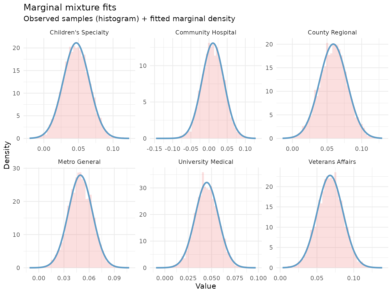

Specify Network-Level Priors

# Based on clinical knowledge:
# - Age effect should be positive but moderate
# - Some heterogeneity expected across hospital types

hierarchical_priors <- list(
  mu = dist_normal(0.05, 0.025),  # Centered on 5% increase per year
  tau = dist_truncated(dist_student_t(3, 0, 0.01), lower = 0)  # Modest heterogeneity
)

# Visualize prior implications
prior_pred <- sample_prior_predictive(
  hierarchical_priors = hierarchical_priors,
  n_groups = 6,
  n_draws = 1000
)

plot(prior_pred, type = "both")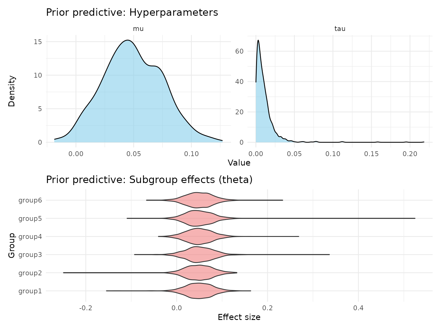

Fit Hierarchical Model

fit_full_post <- shrink(
  mixture = mix,
  hierarchical_priors = hierarchical_priors,
  chains = 4,
  iter = 2000,
  warmup = 1000,
  seed = 123
)

print(fit_full_post)
#> # A tibble: 3 × 7
#>   variable         mean       sd         q2.5       q50    q97.5  rhat
#>   <chr>           <dbl>    <dbl>        <dbl>     <dbl>    <dbl> <dbl>
#> 1 mu          0.0496    0.00717  0.0351       0.0498    0.0636    1.00
#> 2 tau         0.00624   0.00520  0.000263     0.00493   0.0195    1.00
#> 3 tau_squared 0.0000660 0.000119 0.0000000689 0.0000243 0.000381  1.00

# Network-level estimates
mu_tau_full <- extract_mu_tau(fit_full_post)
cat("\nNetwork-level age effect (mu):\n")
#> 
#> Network-level age effect (mu):
cat("  Posterior mean:", round(mean(mu_tau_full$mu), 4), "\n")
#>   Posterior mean: 0.0496
cat("  95% CI: [", round(quantile(mu_tau_full$mu, 0.025), 4), ",",
    round(quantile(mu_tau_full$mu, 0.975), 4), "]\n")
#>   95% CI: [ 0.0351 , 0.0636 ]

cat("\nBetween-site heterogeneity (tau):\n")
#> 
#> Between-site heterogeneity (tau):
cat("  Posterior mean:", round(mean(mu_tau_full$tau), 4), "\n")
#>   Posterior mean: 0.0062
cat("  95% CI: [", round(quantile(mu_tau_full$tau, 0.025), 4), ",",
    round(quantile(mu_tau_full$tau, 0.975), 4), "]\n")
#>   95% CI: [ 3e-04 , 0.0195 ]

Path B: Using Only Summary Statistics

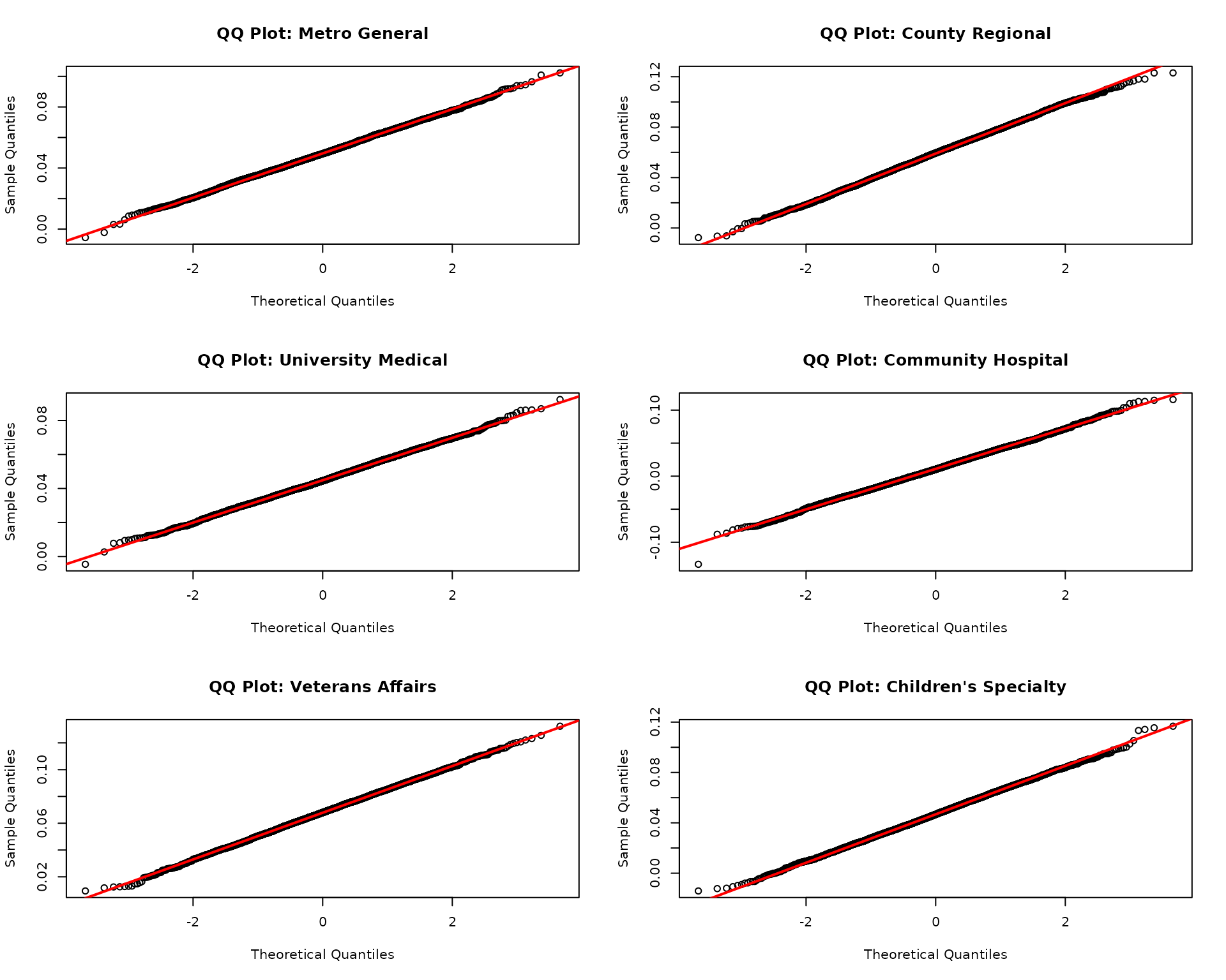
Before using summary statistics, we must verify posteriors are approximately normal.

Step 1: Check Normality Assumption

# Visual checks for approximate normality
oldpar <- par(no.readonly = TRUE)
par(mfrow = c(3, 2))
for(i in 1:6) {
  site_name <- names(site_posteriors)[i]
  samples_i <- as.vector(site_posteriors[[i]])
  
  # QQ plot against normal
  qqnorm(samples_i, main = paste("QQ Plot:", site_name))
  qqline(samples_i, col = "red", lwd = 2)
}

par(oldpar)

# Quantitative checks
normality_checks <- data.frame(
  site = names(site_posteriors),
  skewness = sapply(site_posteriors, function(x) {
    m3 <- mean((x - mean(x))^3)
    s3 <- sd(x)^3
    m3 / s3
  }),
  kurtosis = sapply(site_posteriors, function(x) {
    m4 <- mean((x - mean(x))^4)
    s4 <- sd(x)^4
    m4 / s4 - 3  # Excess kurtosis
  })
)

print(normality_checks)
#>                                      site     skewness     kurtosis
#> Metro General               Metro General  0.006067498  0.009199907
#> County Regional           County Regional -0.050758390 -0.116123944
#> University Medical     University Medical  0.035950881 -0.005600149
#> Community Hospital     Community Hospital  0.008651589  0.118037106
#> Veterans Affairs         Veterans Affairs -0.041185160 -0.015861386
#> Children's Specialty Children's Specialty  0.010783310 -0.090076276

cat("\nNormality assessment:\n")
#> 
#> Normality assessment:
cat("  Skewness close to 0? (|skew| < 0.5 is good)\n")
#>   Skewness close to 0? (|skew| < 0.5 is good)
cat("  Kurtosis close to 0? (|kurt| < 1.0 is good)\n")
#>   Kurtosis close to 0? (|kurt| < 1.0 is good)
cat("  All sites pass:", 
    all(abs(normality_checks$skewness) < 0.5 & abs(normality_checks$kurtosis) < 1.0),
    "\n")
#>   All sites pass: TRUE

Decision rule:

If posteriors look approximately normal, Path B is likely valid
If posteriors are skewed/heavy-tailed, use Path A
If unsure, use Path A

When CLT Fails: A Counter-Example

To illustrate why normality matters, consider a scenario where we are estimating a variance parameter:

# Simulated: posterior for a variance parameter (boundary at 0)
set.seed(999)
variance_posterior <- matrix(rchisq(4000, df = 5) / 5, ncol = 1)

# Compute summary statistics
var_mean <- mean(variance_posterior)
var_se <- sd(variance_posterior)

# Check normality
oldpar <- par(no.readonly = TRUE)
par(mfrow = c(1, 2))
hist(variance_posterior, breaks = 30, main = "Variance Posterior",
     xlab = "sigma^2", col = "lightblue")
qqnorm(variance_posterior, main = "QQ Plot")
qqline(variance_posterior, col = "red", lwd = 2)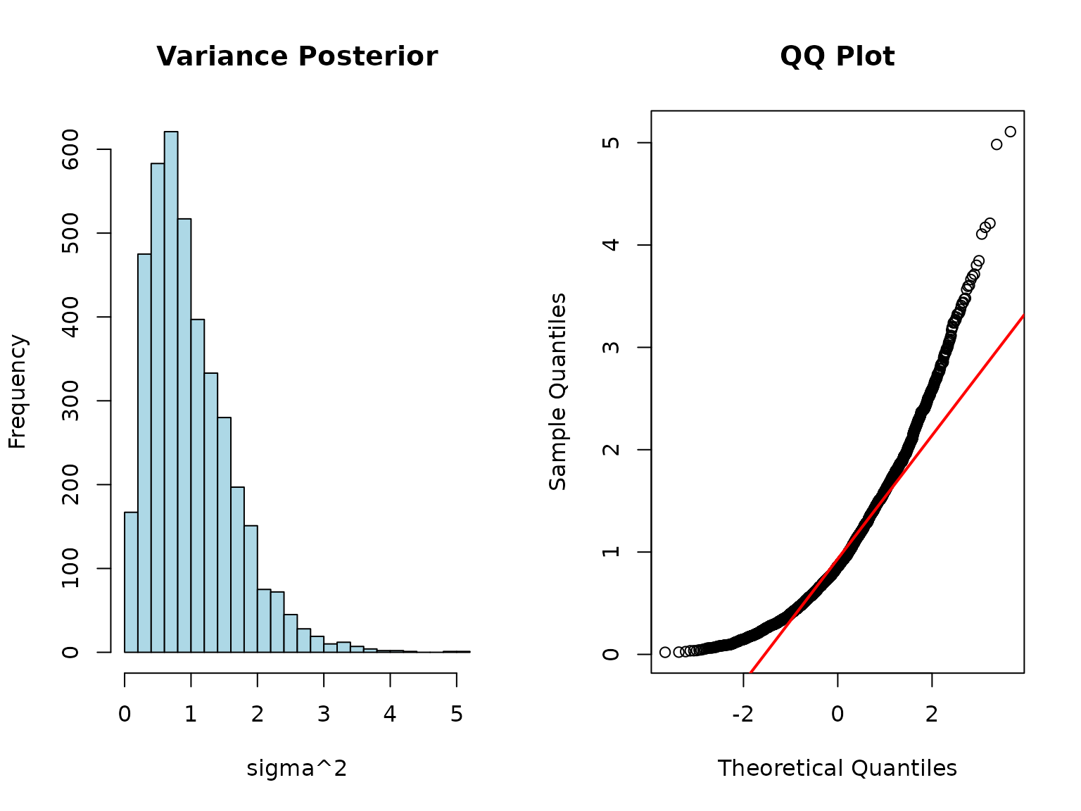

par(oldpar)

# Skewness
skew <- mean((variance_posterior - var_mean)^3) / var_se^3
cat("Skewness:", round(skew, 2), "(should be about 0 for normal)\n")
#> Skewness: 1.24 (should be about 0 for normal)
cat("This posterior is right-skewed - CLT approximation would be poor!\n")
#> This posterior is right-skewed - CLT approximation would be poor!

For this scenario:

Path B summaries would give biased results
Path A mixture handles the skewness correctly

Step 2: Fit Using CLT Approximation

# Extract means and variances
mle_estimates <- site_summaries$beta_age_mean
names(mle_estimates) <- site_summaries$site

mle_variances <- site_summaries$beta_age_se^2
names(mle_variances) <- site_summaries$site

# Fit using MLE path (CLT approximation)
fit_summaries <- shrink(
  mle = mle_estimates,
  var_matrix = mle_variances,
  hierarchical_priors = hierarchical_priors,
  chains = 4,
  iter = 2000,
  warmup = 1000,
  seed = 123,
  verbose = FALSE,
  refresh = 0
)

print(fit_summaries)
#> # A tibble: 3 × 7
#>   variable         mean       sd         q2.5       q50    q97.5  rhat
#>   <chr>           <dbl>    <dbl>        <dbl>     <dbl>    <dbl> <dbl>
#> 1 mu          0.0497    0.00738  0.0351       0.0500    0.0640   1.00 
#> 2 tau         0.00625   0.00522  0.000223     0.00506   0.0189   1.000
#> 3 tau_squared 0.0000663 0.000123 0.0000000498 0.0000256 0.000357 1.000

Compare Paths

mu_tau_summaries <- extract_mu_tau(fit_summaries)

comparison <- data.frame(
  parameter = c("mu", "tau"),
  full_posteriors = c(
    mean(mu_tau_full$mu),
    mean(mu_tau_full$tau)
  ),
  summaries_only = c(
    mean(mu_tau_summaries$mu),
    mean(mu_tau_summaries$tau)
  )
) %>%
  mutate(difference = abs(full_posteriors - summaries_only))

print(comparison)
#>   parameter full_posteriors summaries_only   difference
#> 1        mu     0.049595359    0.049744508 1.491484e-04
#> 2       tau     0.006242385    0.006248864 6.478663e-06

cat("\nMaximum difference:", round(max(comparison$difference), 5), "\n")
#> 
#> Maximum difference: 0.00015

Conclusion: Both paths give nearly identical results because posteriors are approximately normal in this case. This will not always be true.

When each path is appropriate:

Situation	Recommended Path	Reason
Posteriors are normal (verified)	Path B acceptable	CLT holds; minimal sharing
Posteriors are skewed/multimodal	Path A required	CLT fails; mixture needed
Small sample sizes per site	Path A safer	CLT may not hold yet
Boundary constraints	Path A required	CLT assumes interior parameters
Unknown posterior shape	Path A safer	Conservative choice
Maximum privacy needed and normal posteriors	Path B acceptable	But verify normality

Results: Improved Site-Specific Estimates

Visualize Shrinkage Effect

# Using Path A results (nearly identical for Path B)
plot(fit_full_post)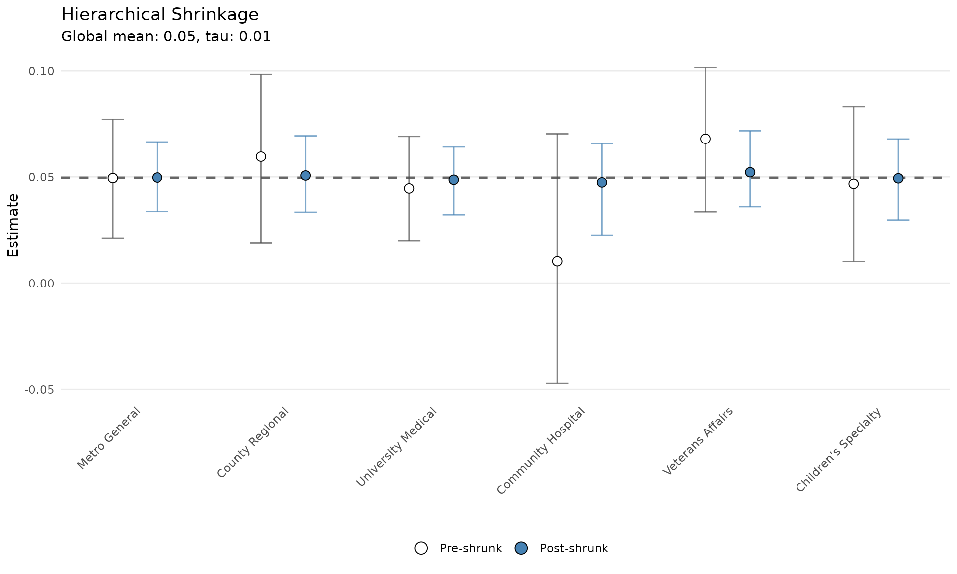

Key insights:

Community Hospital shrinks most toward the network mean
University Medical keeps closest to its original estimate
Metro General and VA Hospital are pulled slightly toward the center
Adaptive borrowing is based on precision

Quantify Uncertainty Reduction

# Get Stage 2 estimates
theta_post <- summarize_theta(fit_full_post)

# Compare Stage 1 vs Stage 2 uncertainty
uncertainty_comparison <- data.frame(
  site = site_summaries$site,
  n_patients = site_summaries$n_patients,
  stage1_se = site_summaries$beta_age_se,
  stage2_se = theta_post$sd
) %>%
  mutate(
    reduction_pct = 100 * (stage1_se - stage2_se) / stage1_se,
    stage1_ci_width = 2 * 1.96 * stage1_se,
    stage2_ci_width = 2 * 1.96 * stage2_se,
    ci_width_reduction = 100 * (stage1_ci_width - stage2_ci_width) / stage1_ci_width
  )

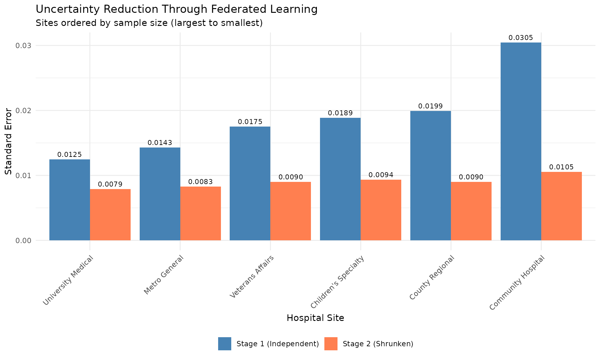
print(uncertainty_comparison)
#>                   site n_patients  stage1_se   stage2_se reduction_pct
#> 1        Metro General       1500 0.01428679 0.008272696      42.09548
#> 2      County Regional        800 0.01992675 0.008979639      54.93675
#> 3   University Medical       2200 0.01246048 0.007916911      36.46382
#> 4   Community Hospital        350 0.03047231 0.010540811      65.40856
#> 5     Veterans Affairs       1100 0.01752091 0.009019055      48.52405
#> 6 Children's Specialty        900 0.01888196 0.009357809      50.44048
#>   stage1_ci_width stage2_ci_width ci_width_reduction
#> 1      0.05600421      0.03242897           42.09548
#> 2      0.07811285      0.03520019           54.93675
#> 3      0.04884507      0.03103429           36.46382
#> 4      0.11945147      0.04131998           65.40856
#> 5      0.06868197      0.03535470           48.52405
#> 6      0.07401729      0.03668261           50.44048

Largest improvements occur in smaller sites.

Visualize Uncertainty Reduction

# Prepare data for plotting
uncertainty_long <- uncertainty_comparison %>%
  select(site, n_patients, stage1_se, stage2_se) %>%
  pivot_longer(
    cols = c(stage1_se, stage2_se),
    names_to = "stage",
    values_to = "standard_error"
  ) %>%
  mutate(
    stage = factor(stage, 
                   levels = c("stage1_se", "stage2_se"),
                   labels = c("Stage 1 (Independent)", "Stage 2 (Shrunken)"))
  )

ggplot(uncertainty_long, aes(x = reorder(site, -n_patients), y = standard_error, 
                              fill = stage)) +
  geom_col(position = "dodge") +
  geom_text(aes(label = sprintf("%.4f", standard_error)),
            position = position_dodge(width = 0.9),
            vjust = -0.5, size = 3) +
  scale_fill_manual(values = c("Stage 1 (Independent)" = "steelblue",
                               "Stage 2 (Shrunken)" = "coral")) +
  labs(
    title = "Uncertainty Reduction Through Federated Learning",
    subtitle = "Sites ordered by sample size (largest to smallest)",
    x = "Hospital Site",
    y = "Standard Error",
    fill = NULL
  ) +
  theme_minimal() +
  theme(
    axis.text.x = element_text(angle = 45, hjust = 1),
    legend.position = "bottom"
  )

Clinical Impact: Network-Calibrated Predictions

Stage 1: Independent Site Predictions

# Example: 70-year-old patient
age <- 70
baseline_age <- 60  # Reference age

# Stage 1 predictions (independent)
stage1_log_or <- site_summaries$beta_age_mean * (age - baseline_age)
stage1_or <- exp(stage1_log_or)

stage1_preds <- data.frame(
  site = site_summaries$site,
  log_or = stage1_log_or,
  odds_ratio = stage1_or,
  stage = "Independent"
)

Stage 2: Network-Calibrated Predictions

# Stage 2 predictions (network-calibrated)
stage2_log_or <- theta_post$mean * (age - baseline_age)
stage2_or <- exp(stage2_log_or)

stage2_preds <- data.frame(
  site = theta_post$group,
  log_or = stage2_log_or,
  odds_ratio = stage2_or,
  stage = "Network-Calibrated"
)

# Combine
all_preds <- rbind(stage1_preds, stage2_preds)

Visualize Prediction Changes

ggplot(all_preds, aes(x = site, y = odds_ratio, fill = stage)) +
  geom_col(position = "dodge") +
  geom_hline(yintercept = 1, linetype = "dashed", color = "gray30") +
  geom_text(aes(label = sprintf("%.2f", odds_ratio)),
            position = position_dodge(width = 0.9),
            vjust = -0.5, size = 3) +
  scale_fill_manual(values = c("Independent" = "steelblue",
                               "Network-Calibrated" = "coral")) +
  labs(
    title = "Predicted Odds Ratio for 70 vs 60 Year-Old Patient",
    subtitle = "Network calibration stabilizes predictions across sites",
    x = "Hospital Site",
    y = "Odds Ratio",
    fill = NULL
  ) +
  theme_minimal() +
  theme(
    axis.text.x = element_text(angle = 45, hjust = 1),
    legend.position = "bottom"
  )

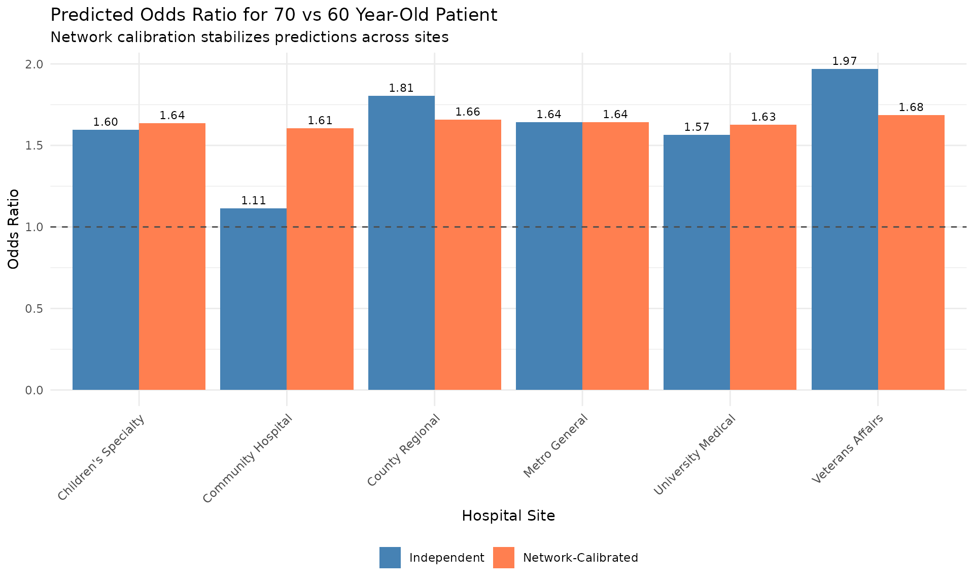
Clinical interpretation:

Independent estimates vary across sites
Network-calibrated estimates are more consistent
Small sites benefit most from network information
Meaningful site-specific variation is preserved

Privacy-Preserving Benefits

What Gets Shared

privacy_comparison <- data.frame(
  approach = c("Centralized Data", "Path A: Full Posteriors", "Path B: Summaries"),
  patient_data_shared = c("Yes - All records", "No", "No"),
  data_per_site = c("about 50-200 MB", "about 200 KB", "about 16 bytes"),
  privacy_risk = c("High", "Low", "Minimal"),
  validity = c("N/A", "Always valid", "Only if CLT holds"),
  when_to_use = c("Not for federated", "Default choice", "When posteriors normal")
)

knitr::kable(privacy_comparison, align = "lccccl")

approach	patient_data_shared	data_per_site	privacy_risk	validity	when_to_use
Centralized Data	Yes - All records	about 50-200 MB	High	N/A	Not for federated
Path A: Full Posteriors	No	about 200 KB	Low	Always valid	Default choice
Path B: Summaries	No	about 16 bytes	Minimal	Only if CLT holds	When posteriors normal

Key insight: Path A shares much less data than centralized analysis while being valid in all scenarios. Path B shares even less data but requires approximate posterior normality.

Compliance Benefits

Certain data privacy policies satisfied:

No patient-level data leaves sites
Only aggregate statistical summaries are shared
De-identified parameter estimates are exchanged

Advanced Federated Scenarios

Scenario 1: Heterogeneous Models

Sites use different model specifications:

# Site 1: Linear model
# Site 2: GLM with splines
# Site 3: Bayesian hierarchical model

# As long as they all estimate the same parameter, shrinkr can combine them.

samples_heterogeneous <- list(
  site1 = samples_from_lm,
  site2 = samples_from_glm,
  site3 = samples_from_bayes
)

# Proceed with shrinkr as usual
mix <- fit_mixture(samples_heterogeneous, K_max = 3)
fit <- shrink(mix, hierarchical_priors = priors)

Scenario 2: Meta-Analysis of Published Studies

Combine published results without raw data:

# Extracted from publications
published_estimates <- c(
  "Smith et al. (2020)" = 0.45,
  "Jones et al. (2021)" = 0.52,
  "Garcia et al. (2022)" = 0.38,
  "Williams et al. (2023)" = 0.48
)

published_ses <- c(0.12, 0.15, 0.10, 0.13)

# Apply shrinkr for Bayesian meta-analysis
# NOTE: This assumes published estimates are approximately normal.

fit_meta <- shrink(
  mle = published_estimates,
  var_matrix = published_ses^2,
  hierarchical_priors = priors
)

Scenario 3: Iterative Federated Updates

New sites join the network over time:

# Initial network
fit_initial <- shrink(samples_initial, priors)

# New site joins
samples_updated <- c(samples_initial, list(new_site = new_samples))
fit_updated <- shrink(samples_updated, priors)

# Compare network estimates before/after
mu_before <- mean(extract_mu_tau(fit_initial)$mu)
mu_after <- mean(extract_mu_tau(fit_updated)$mu)

Federated Learning Best Practices

1. Establish Data Governance

Before sharing any summaries:

Define what parameters will be shared
Establish data use agreements for summary statistics
Document privacy protections
Get institutional approval

2. Standardize Stage 1 Models

Ensure comparability:

Use consistent outcome definitions
Standardize predictor coding/scaling
Document any site-specific modifications
Agree on parameter naming conventions

3. Verify Normality if Using Summaries

If using Path B, sites must:

Generate QQ plots of posteriors
Compute skewness and excess kurtosis
Share diagnostic plots with the coordinator
Agree normality is reasonable before proceeding

Red flags for non-normality:

Boundary constraints, such as variance parameters or probabilities
Small sample sizes
Highly skewed or heavy-tailed data

When in doubt, use Path A.

4. Quality Control

Central coordinator should:

Check for outliers in shared summaries
Verify mixture approximation quality for Path A
Assess prior-data conflicts
Report back site-specific diagnostics

# Example: Flag suspicious estimates
qc_results <- site_summaries %>%
  mutate(
    z_score = (beta_age_mean - median(beta_age_mean)) / mad(beta_age_mean),
    flag = ifelse(abs(z_score) > 3, "Review", "OK")
  )

cat("Quality control flags:\n")
#> Quality control flags:
print(qc_results %>% select(site, beta_age_mean, z_score, flag))
#>                                      site beta_age_mean    z_score   flag
#> Metro General               Metro General    0.04958522  0.1321992     OK
#> County Regional           County Regional    0.05905738  1.0300204     OK
#> University Medical     University Medical    0.04482541 -0.3189611     OK
#> Community Hospital     Community Hospital    0.01077674 -3.5462732 Review
#> Veterans Affairs         Veterans Affairs    0.06783668  1.8621681     OK
#> Children's Specialty Children's Specialty    0.04679578 -0.1321992     OK

5. Sensitivity Analysis

Test robustness to prior specifications:

# Alternative prior: More heterogeneity
priors_alt <- list(
  mu = dist_normal(0.05, 0.025),
  tau = dist_truncated(dist_student_t(3, 0, 0.02), lower = 0)
)

fit_alt <- shrink(
  mixture = mix,
  hierarchical_priors = priors_alt,
  chains = 2,
  iter = 1000,
  warmup = 500,
  seed = 456
)

# Compare key results
mu_base <- mean(extract_mu_tau(fit_full_post)$mu)
mu_alt <- mean(extract_mu_tau(fit_alt)$mu)

tau_base <- mean(extract_mu_tau(fit_full_post)$tau)
tau_alt <- mean(extract_mu_tau(fit_alt)$tau)

cat("Sensitivity to prior on tau:\n")
#> Sensitivity to prior on tau:
cat("  mu: Base =", round(mu_base, 4), ", Alternative =", round(mu_alt, 4), "\n")
#>   mu: Base = 0.0496 , Alternative = 0.0502
cat("  tau: Base =", round(tau_base, 4), ", Alternative =", round(tau_alt, 4), "\n")
#>   tau: Base = 0.0062 , Alternative = 0.0085

6. Transparent Reporting

Share with network participants:

Network-level estimates
Site-specific shrunken estimates
Diagnostics, including convergence and sensitivity
Quantified uncertainty reduction

# Create site-specific report
site_report <- data.frame(
  site = theta_post$group,
  original_estimate = site_summaries$beta_age_mean,
  original_se = site_summaries$beta_age_se,
  calibrated_estimate = theta_post$mean,
  calibrated_se = theta_post$sd,
  uncertainty_reduction = uncertainty_comparison$reduction_pct
) %>%
  mutate(across(where(is.numeric), ~round(.x, 4)))

cat("\nFederated Learning Results Report\n")
#> 
#> Federated Learning Results Report
cat("==================================\n\n")
#> ==================================
cat("Network-level estimate (mu):", round(mean(mu_tau_full$mu), 4), "\n")
#> Network-level estimate (mu): 0.0496
cat("Between-site heterogeneity (tau):", round(mean(mu_tau_full$tau), 4), "\n\n")
#> Between-site heterogeneity (tau): 0.0062
cat("Site-specific calibrated estimates:\n")
#> Site-specific calibrated estimates:
print(site_report)
#>                   site original_estimate original_se calibrated_estimate
#> 1        Metro General            0.0496      0.0143              0.0497
#> 2      County Regional            0.0591      0.0199              0.0506
#> 3   University Medical            0.0448      0.0125              0.0486
#> 4   Community Hospital            0.0108      0.0305              0.0474
#> 5     Veterans Affairs            0.0678      0.0175              0.0522
#> 6 Children's Specialty            0.0468      0.0189              0.0493
#>   calibrated_se uncertainty_reduction
#> 1        0.0083               42.0955
#> 2        0.0090               54.9368
#> 3        0.0079               36.4638
#> 4        0.0105               65.4086
#> 5        0.0090               48.5241
#> 6        0.0094               50.4405

Advantages of shrinkr for Federated Learning

Feature	Benefit
Two-stage design	Clean separation between local Stage 1 and collaborative Stage 2 analysis
Flexible sharing options	Can share full posteriors, mixture approximations, or summaries if CLT holds
Privacy preserving	No patient-level data exposure
Flexible Stage 1	Each site can use their preferred modeling approach
Transparent shrinkage	Sites understand how their estimates are adjusted
Uncertainty quantification	Proper propagation of both within-site and between-site uncertainty
Handles non-normality	Mixture approximation works for skewed or multimodal posteriors
Regulatory friendly	Supports HIPAA, GDPR, and institutional privacy constraints

When to Use Federated shrinkr

Ideal scenarios:

Multi-center clinical trials
Hospital network collaborations
International consortia
Meta-analyses with limited published data
Any setting where data cannot be centralized

Requirements:

Sites can fit Bayesian models independently
Sites can share posterior samples or mixture approximations
Or sites can share means and SEs and posteriors are approximately normal
Common parameter of interest across sites
Central coordinator to run Stage 2

Not recommended when:

Sites have very different populations
Sites cannot agree on parameter definitions
Posteriors are highly non-normal and sites cannot share full posteriors or mixtures

Summary

The shrinkr package enables privacy-preserving federated learning through its two-stage design:

Stage 1: Fit local models behind each site’s firewall
Check normality: Verify CLT assumptions if using summaries
Share: Full posteriors, mixtures, or summaries
Stage 2: Apply hierarchical shrinkage centrally
Return: Improved site-specific estimates

Key advantages:

Data sovereignty preserved
Flexible sharing options
Handles non-normal posteriors via mixture approximation
Improved estimates for all sites
Proper uncertainty quantification
Compatible with privacy-focused workflows

Critical decision: Which path?

Path A: Always valid and handles any posterior shape
Path B: Valid only if posteriors are approximately normal
When uncertain: Use Path A

Additional Resources

# See also:
vignette("getting_started")
vignette("tidy_bayesian_workflow")
vignette("brms_integration")

Session Info

sessionInfo()
#> R version 4.6.1 (2026-06-24)
#> Platform: x86_64-pc-linux-gnu
#> Running under: Ubuntu 24.04.4 LTS
#> 
#> Matrix products: default
#> BLAS:   /usr/lib/x86_64-linux-gnu/openblas-pthread/libblas.so.3 
#> LAPACK: /usr/lib/x86_64-linux-gnu/openblas-pthread/libopenblasp-r0.3.26.so;  LAPACK version 3.12.0
#> 
#> locale:
#>  [1] LC_CTYPE=C.UTF-8       LC_NUMERIC=C           LC_TIME=C.UTF-8       
#>  [4] LC_COLLATE=C.UTF-8     LC_MONETARY=C.UTF-8    LC_MESSAGES=C.UTF-8   
#>  [7] LC_PAPER=C.UTF-8       LC_NAME=C              LC_ADDRESS=C          
#> [10] LC_TELEPHONE=C         LC_MEASUREMENT=C.UTF-8 LC_IDENTIFICATION=C   
#> 
#> time zone: UTC
#> tzcode source: system (glibc)
#> 
#> attached base packages:
#> [1] stats     graphics  grDevices utils     datasets  methods   base     
#> 
#> other attached packages:
#> [1] tidyr_1.3.2          ggplot2_4.0.3        dplyr_1.2.1         
#> [4] posterior_1.7.0      distributional_0.8.1 shrinkr_0.4.5       
#> 
#> loaded via a namespace (and not attached):
#>  [1] tensorA_0.36.2.1      utf8_1.2.6            sass_0.4.10          
#>  [4] generics_0.1.4        digest_0.6.39         magrittr_2.0.5       
#>  [7] evaluate_1.0.5        grid_4.6.1            RColorBrewer_1.1-3   
#> [10] fastmap_1.2.0         jsonlite_2.0.0        pkgbuild_1.4.8       
#> [13] backports_1.5.1       mclust_6.1.2          gridExtra_2.3.1      
#> [16] purrr_1.2.2           QuickJSR_1.10.0       scales_1.4.0         
#> [19] codetools_0.2-20      textshaping_1.0.5     jquerylib_0.1.4      
#> [22] abind_1.4-8           cli_3.6.6             rlang_1.2.0          
#> [25] withr_3.0.3           cachem_1.1.0          yaml_2.3.12          
#> [28] otel_0.2.0            StanHeaders_2.32.10   tools_4.6.1          
#> [31] rstan_2.32.7          inline_0.3.21         parallel_4.6.1       
#> [34] rstantools_2.6.0      checkmate_2.3.4       vctrs_0.7.3          
#> [37] R6_2.6.1              matrixStats_1.5.0     stats4_4.6.1         
#> [40] lifecycle_1.0.5       fs_2.1.0              htmlwidgets_1.6.4    
#> [43] ragg_1.5.2            pkgconfig_2.0.3       desc_1.4.3           
#> [46] pkgdown_2.2.0         RcppParallel_5.1.11-2 bslib_0.11.0         
#> [49] pillar_1.11.1         gtable_0.3.6          loo_2.10.0           
#> [52] glue_1.8.1            Rcpp_1.1.1-1.1        systemfonts_1.3.2    
#> [55] xfun_0.59             tibble_3.3.1          tidyselect_1.2.1     
#> [58] knitr_1.51            farver_2.1.2          patchwork_1.3.2      
#> [61] htmltools_0.5.9       labeling_0.4.3        rmarkdown_2.31       
#> [64] compiler_4.6.1        S7_0.2.2

Jacob M. Maronge

2026-07-06