Survival Analysis with brms and shrinkr

Jacob M. Maronge

2026-07-06

Overview

This vignette demonstrates hierarchical shrinkage for survival analysis using the classic veteran lung cancer dataset. We explore a key clinical question: Does the treatment effect vary by lung cancer cell type?

Rather than treating cell type-specific treatment effects as fixed interaction terms, we model them as random effects drawn from a common distribution. This hierarchical structure allows us to:

• Borrow strength across cell types, especially for small subgroups
• Estimate the overall mean treatment effect (mu)
• Quantify heterogeneity in treatment effects (tau)
• Shrink extreme subgroup estimates toward the group mean

We compare three modeling approaches:

1. Two-stage (brms + shrinkr): fit a Cox model in brms, then apply hierarchical shrinkage in shrinkr
2. Full hierarchical (brms): fit the hierarchical Cox model in one step
3. Two-stage (frequentist + shrinkr): use Cox model estimates from survival::coxph(), then apply shrinkage

The two-stage brms workflow produces nearly identical results to the full hierarchical model, while making it easy to explore alternative hierarchical priors without repeatedly refitting the Stage 1 model.

Some model-fitting steps are computationally intensive and are not evaluated during routine package checks. All code needed to reproduce the analysis is shown below.

Setup

library(shrinkr)
library(brms)
library(tidybayes)
library(distributional)
library(tidyverse)
library(survival)
library(posterior)
library(patchwork)

theme_set(theme_minimal(base_size = 12))

cell_types <- c("squamous", "smallcell", "adeno", "large")

prior_specs <- list(
  very_strong = list(name = "Very Strong", scale = 0.1),
  strong = list(name = "Strong", scale = 0.25),
  moderate = list(name = "Moderate", scale = 0.5),
  weak = list(name = "Weak", scale = 1.0),
  very_weak = list(name = "Very Weak", scale = 2.0)
)

The Veteran Dataset

data(veteran, package = "survival")

head(veteran)
#>   trt celltype time status karno diagtime age prior
#> 1   1 squamous   72      1    60        7  69     0
#> 2   1 squamous  411      1    70        5  64    10
#> 3   1 squamous  228      1    60        3  38     0
#> 4   1 squamous  126      1    60        9  63    10
#> 5   1 squamous  118      1    70       11  65    10
#> 6   1 squamous   10      1    20        5  49     0
table(veteran$celltype, veteran$trt)
#>            
#>              1  2
#>   squamous  15 20
#>   smallcell 30 18
#>   adeno      9 18
#>   large     15 12

veteran %>%
  group_by(celltype, trt) %>%
  summarise(
    n = n(),
    deaths = sum(status),
    median_time = median(time),
    .groups = "drop"
  )
#> # A tibble: 8 × 5
#>   celltype    trt     n deaths median_time
#>   <fct>     <dbl> <int>  <dbl>       <dbl>
#> 1 squamous      1    15     13       100  
#> 2 squamous      2    20     18       156. 
#> 3 smallcell     1    30     28        53  
#> 4 smallcell     2    18     17        27  
#> 5 adeno         1     9      9        92  
#> 6 adeno         2    18     17        49.5
#> 7 large         1    15     14       177  
#> 8 large         2    12     12        82

Variables:

• time: survival time (days)
• status: death indicator (1 = died)
• trt: treatment (1 = standard, 2 = test)
• celltype: cancer type (squamous, smallcell, adeno, large)
• karno: Karnofsky score (performance status)
• age: age in years

The dataset contains 137 patients across four cell types, with varying sample sizes.

Approach 1: Two-Stage (brms + shrinkr)

Stage 1: Fit Cox Model

We begin by fitting a Cox proportional hazards model that allows the treatment effect to vary by cell type. At this stage we estimate subgroup-specific treatment effects without adding hierarchical shrinkage across cell types. That hierarchical regularization is introduced in Stage 2.

brms_uninformative <- brm(
  time | cens(1 - status) ~ trt:celltype + karno + age,
  data = veteran,
  family = cox(),
  chains = 4,
  iter = 4000,
  warmup = 1000,
  seed = 123
)

brms_uninformative_summary <- capture.output(print(summary(brms_uninformative)))

What this model does:

• Estimates a separate log hazard ratio for the test treatment in each cell type
• Adjusts for baseline performance status (karno) and age
• Leaves pooling across cell types to the second-stage hierarchical model

Results:

cat(brms_uninformative_summary, sep = "\n")
#>  Family: cox 
#>   Links: mu = log 
#> Formula: time | cens(1 - status) ~ trt:celltype + karno + age 
#>    Data: veteran (Number of observations: 137) 
#>   Draws: 4 chains, each with iter = 4000; warmup = 1000; thin = 1;
#>          total post-warmup draws = 12000
#> 
#> Regression Coefficients:
#>                       Estimate Est.Error l-95% CI
#> Intercept                 4.16      0.74     2.70
#> karno                    -0.03      0.01    -0.04
#> age                      -0.01      0.01    -0.02
#> trt:celltypesquamous     -0.12      0.21    -0.52
#> trt:celltypesmallcell     0.51      0.23     0.05
#> trt:celltypeadeno         0.54      0.20     0.13
#> trt:celltypelarge         0.16      0.23    -0.31
#>                       u-95% CI Rhat Bulk_ESS Tail_ESS
#> Intercept                 5.61 1.00     9000     8957
#> karno                    -0.02 1.00    11647     9539
#> age                       0.01 1.00     9875     8676
#> trt:celltypesquamous      0.29 1.00     5515     7429
#> trt:celltypesmallcell     0.95 1.00     5310     7315
#> trt:celltypeadeno         0.94 1.00     5398     7230
#> trt:celltypelarge         0.61 1.00     5399     7077
#> 
#> Draws were sampled using sampling(NUTS). For each parameter, Bulk_ESS
#> and Tail_ESS are effective sample size measures, and Rhat is the potential
#> scale reduction factor on split chains (at convergence, Rhat = 1).

Stage 2: Apply Hierarchical Shrinkage

Now we extract the cell type-specific treatment effect posteriors and apply hierarchical shrinkage.

Step 1: Extract posterior samples

brms_posteriors <- brms_uninformative %>%
  spread_draws(`b_trt:celltypesquamous`, `b_trt:celltypesmallcell`,
               `b_trt:celltypeadeno`, `b_trt:celltypelarge`) %>%
  select(-c(.chain, .iteration, .draw)) %>%
  pivot_longer(everything(), names_to = "celltype", values_to = "value") %>%
  mutate(celltype = gsub("b_trt:celltype", "", celltype)) %>%
  group_by(celltype) %>%
  summarise(draws = list(matrix(value, ncol = 1)), .groups = "drop") %>%
  deframe()

brms_posteriors is a named list containing posterior draws for each cell type.

Step 2: Fit a Gaussian mixture approximation

The fit_mixture() function approximates each subgroup posterior with a mixture of Gaussian components. This creates a flexible representation of the Stage 1 posterior that can be passed to shrink().

mix_brms <- fit_mixture(brms_posteriors, K_max = 3, verbose = TRUE)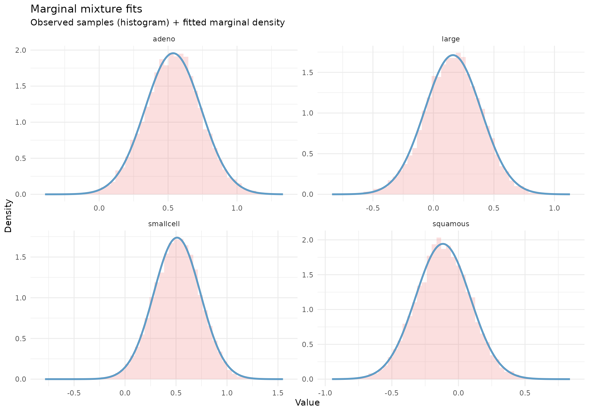

print(mix_brms)
plot(mix_brms, draws = brms_posteriors)

Understanding the mixture approximation:

• Each posterior is approximated as a weighted sum of Gaussian components
• The number of components is chosen separately for each cell type
• This allows the approximation to capture skewness or heavier tails when needed

Step 3: Apply a hierarchical prior

priors_moderate <- list(
  mu = dist_normal(0, 1),
  tau = dist_truncated(dist_normal(0, 0.5), lower = 0)
)

fit_twostage_brms <- shrink(
  mixture = mix_brms,
  hierarchical_priors = priors_moderate,
  chains = 4,
  iter = 4000,
  warmup = 1000,
  seed = 456
)

moderate_brms_output <- capture.output(print(fit_twostage_brms))

Results:

cat(moderate_brms_output, sep = "\n")
#> # A tibble: 3 × 7
#>   variable     mean    sd    q2.5   q50 q97.5  rhat
#>   <chr>       <dbl> <dbl>   <dbl> <dbl> <dbl> <dbl>
#> 1 mu          0.246 0.265 -0.272  0.245 0.757  1.00
#> 2 tau         0.361 0.176  0.123  0.324 0.812  1.00
#> 3 tau_squared 0.161 0.177  0.0150 0.105 0.659  1.00

Interpreting the shrinkage:

• Cell type-specific estimates are pulled toward the overall mean (mu)
• The amount of shrinkage depends on tau, the between-cell-type heterogeneity
• Smaller tau implies stronger pooling
• Larger tau implies weaker pooling

Approach 2: Full Hierarchical (brms)

For comparison, we fit the corresponding one-stage hierarchical Cox model directly in brms.

brms_hierarchical <- brm(
  time | cens(1 - status) ~ trt + (0 + trt | celltype) + karno + age,
  data = veteran,
  family = cox(),
  prior = c(
    prior(normal(0, 1), class = b, coef = "trt"),
    prior(normal(0, 0.5), class = sd, group = "celltype", lb = 0)
  ),
  chains = 4,
  iter = 4000,
  warmup = 1000,
  seed = 123
)

brms_hierarchical_summary <- capture.output(print(summary(brms_hierarchical)))

brms_hier_effects <- brms_hierarchical %>%
  spread_draws(r_celltype[celltype, term], b_trt) %>%
  filter(term == "trt") %>%
  mutate(theta = b_trt + r_celltype) %>%
  group_by(celltype) %>%
  summarise(
    hr_mean = exp(mean(theta)),
    hr_lower = exp(quantile(theta, 0.025)),
    hr_upper = exp(quantile(theta, 0.975)),
    .groups = "drop"
  )

Results:

cat(brms_hierarchical_summary, sep = "\n")
#>  Family: cox 
#>   Links: mu = log 
#> Formula: time | cens(1 - status) ~ trt + (0 + trt | celltype) + karno + age 
#>    Data: veteran (Number of observations: 137) 
#>   Draws: 4 chains, each with iter = 4000; warmup = 1000; thin = 1;
#>          total post-warmup draws = 12000
#> 
#> Multilevel Hyperparameters:
#> ~celltype (Number of levels: 4) 
#>         Estimate Est.Error l-95% CI u-95% CI Rhat
#> sd(trt)     0.36      0.18     0.13     0.80 1.00
#>         Bulk_ESS Tail_ESS
#> sd(trt)     4188     6657
#> 
#> Regression Coefficients:
#>           Estimate Est.Error l-95% CI u-95% CI Rhat
#> Intercept     4.11      0.74     2.66     5.55 1.00
#> trt           0.26      0.26    -0.24     0.79 1.00
#> karno        -0.03      0.01    -0.04    -0.02 1.00
#> age          -0.01      0.01    -0.02     0.01 1.00
#>           Bulk_ESS Tail_ESS
#> Intercept    11705     9033
#> trt           5386     6740
#> karno        13722     9846
#> age          11879     7469
#> 
#> Draws were sampled using sampling(NUTS). For each parameter, Bulk_ESS
#> and Tail_ESS are effective sample size measures, and Rhat is the potential
#> scale reduction factor on split chains (at convergence, Rhat = 1).

Approach 3: Two-Stage (Frequentist + shrinkr)

We can also apply the second-stage shrinkage model to standard Cox model estimates and their covariance matrix.

cox_model <- coxph(
  Surv(time, status) ~ trt:celltype + karno + age,
  data = veteran
)

cox_summary <- summary(cox_model)

trt_idx <- grep("^trt:celltype", names(coef(cox_model)))

trt_effects <- coef(cox_model)[trt_idx]
trt_vcov <- vcov(cox_model)[trt_idx, trt_idx, drop = FALSE]

names(trt_effects) <- gsub("^trt:celltype", "", names(trt_effects))
rownames(trt_vcov) <- colnames(trt_vcov) <- names(trt_effects)

print(cox_summary)
#> Call:
#> coxph(formula = Surv(time, status) ~ trt:celltype + karno + age, 
#>     data = veteran)
#> 
#>   n= 137, number of events= 128 
#> 
#>                            coef exp(coef)  se(coef)      z Pr(>|z|)    
#> karno                 -0.031511  0.968980  0.005412 -5.823  5.8e-09 ***
#> age                   -0.009056  0.990985  0.009125 -0.992  0.32102    
#> trt:celltypesquamous  -0.058593  0.943091  0.210626 -0.278  0.78087    
#> trt:celltypesmallcell  0.585704  1.796254  0.238641  2.454  0.01411 *  
#> trt:celltypeadeno      0.626150  1.870396  0.210631  2.973  0.00295 ** 
#> trt:celltypelarge      0.236620  1.266960  0.237554  0.996  0.31922    
#> ---
#> Signif. codes:  0 '***' 0.001 '**' 0.01 '*' 0.05 '.' 0.1 ' ' 1
#> 
#>                       exp(coef) exp(-coef) lower .95 upper .95
#> karno                    0.9690     1.0320    0.9588    0.9793
#> age                      0.9910     1.0091    0.9734    1.0089
#> trt:celltypesquamous     0.9431     1.0603    0.6241    1.4251
#> trt:celltypesmallcell    1.7963     0.5567    1.1252    2.8675
#> trt:celltypeadeno        1.8704     0.5346    1.2378    2.8263
#> trt:celltypelarge        1.2670     0.7893    0.7953    2.0182
#> 
#> Concordance= 0.733  (se = 0.021 )
#> Likelihood ratio test= 63.27  on 6 df,   p=1e-11
#> Wald test            = 62.9  on 6 df,   p=1e-11
#> Score (logrank) test = 67.8  on 6 df,   p=1e-12

print("Treatment effects (log HR):")
#> [1] "Treatment effects (log HR):"
print(trt_effects)
#>   squamous  smallcell      adeno      large 
#> -0.0585926  0.5857036  0.6261501  0.2366201

print("\nStandard errors:")
#> [1] "\nStandard errors:"
print(sqrt(diag(trt_vcov)))
#>  squamous smallcell     adeno     large 
#> 0.2106261 0.2386409 0.2106312 0.2375536

fit_twostage_freq <- shrink(
  mle = trt_effects,
  var_matrix = trt_vcov,
  hierarchical_priors = priors_moderate,
  chains = 4,
  iter = 4000,
  warmup = 1000,
  seed = 456
)

moderate_freq_output <- capture.output(print(fit_twostage_freq))

Results:

cat(moderate_freq_output, sep = "\n")
#> # A tibble: 3 × 7
#>   variable     mean    sd    q2.5   q50 q97.5  rhat
#>   <chr>       <dbl> <dbl>   <dbl> <dbl> <dbl> <dbl>
#> 1 mu          0.313 0.266 -0.218  0.312 0.834  1.00
#> 2 tau         0.369 0.178  0.127  0.334 0.822  1.00
#> 3 tau_squared 0.168 0.182  0.0160 0.112 0.675  1.00

Compare Three Approaches

Numerical comparison

theta_brms <- summary(fit_twostage_brms)$theta %>%
  transmute(
    celltype = group,
    twostage_brms = mean
  )

theta_freq <- summary(fit_twostage_freq)$theta %>%
  transmute(
    celltype = group,
    twostage_freq = mean
  )

comparison <- brms_hier_effects %>%
  transmute(
    celltype,
    full_hier_brms = log(hr_mean)
  ) %>%
  left_join(theta_brms, by = "celltype") %>%
  left_join(theta_freq, by = "celltype") %>%
  mutate(
    diff_two_stage_vs_full = twostage_brms - full_hier_brms
  )

knitr::kable(
  comparison[, 1:4],
  digits = 3,
  caption = "Comparison of treatment effects (log HR scale)"
)

Comparison of treatment effects (log HR scale)

celltype	brms_hierarchical	brms_shrinkr	freq_shrinkr
squamous	-0.072	-0.067	-0.016
smallcell	0.450	0.454	0.522
adeno	0.472	0.472	0.557
large	0.164	0.167	0.233

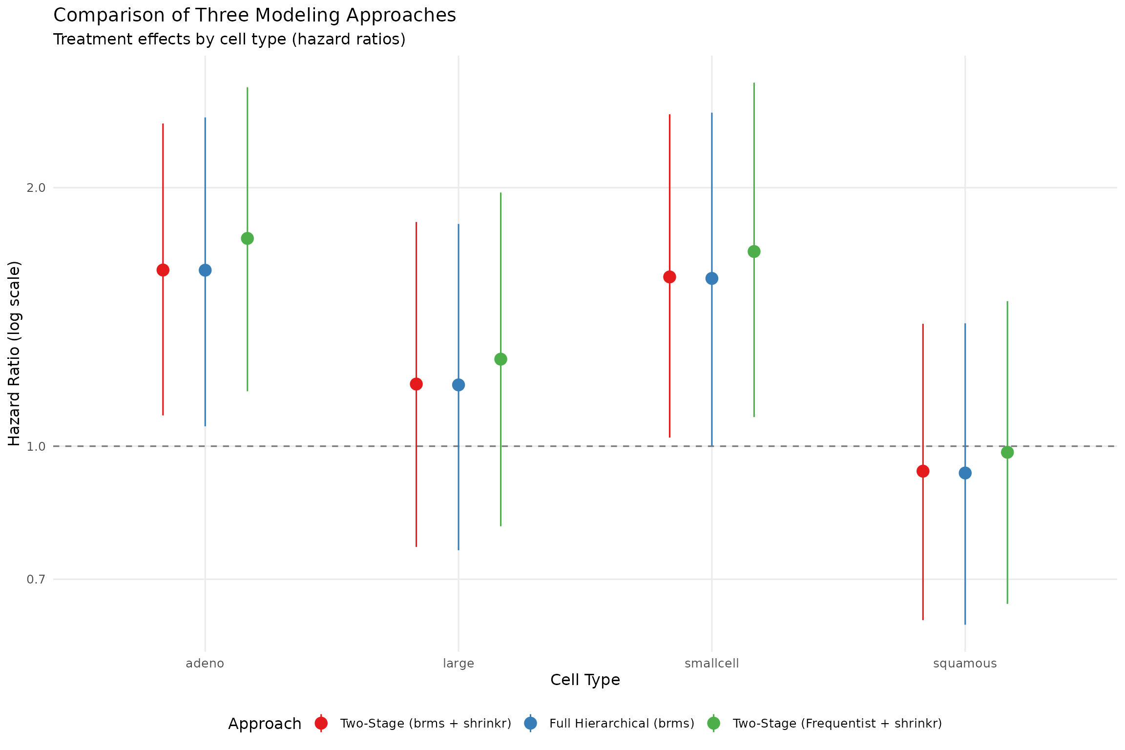
Key observations:

• The two-stage brms + shrinkr and full hierarchical brms fits are nearly identical
• This supports the equivalence of the two formulations in this example
• The frequentist Stage 1 approach differs modestly because the first-stage estimates differ
• All approaches show shrinkage toward a common mean

Visual comparison

theta_brms_plot <- summary(fit_twostage_brms)$theta %>%
  mutate(
    approach = "Two-Stage (brms + shrinkr)",
    hr_mean = exp(mean),
    hr_lower = exp(q2.5),
    hr_upper = exp(q97.5),
    celltype = group
  ) %>%
  select(celltype, approach, hr_mean, hr_lower, hr_upper)

theta_freq_plot <- summary(fit_twostage_freq)$theta %>%
  mutate(
    approach = "Two-Stage (Frequentist + shrinkr)",
    hr_mean = exp(mean),
    hr_lower = exp(q2.5),
    hr_upper = exp(q97.5),
    celltype = group
  ) %>%
  select(celltype, approach, hr_mean, hr_lower, hr_upper)

all_approaches <- bind_rows(
  theta_brms_plot,
  brms_hier_effects %>% mutate(approach = "Full Hierarchical (brms)"),
  theta_freq_plot
) %>%
  mutate(
    approach = factor(approach, levels = c(
      "Two-Stage (brms + shrinkr)",
      "Full Hierarchical (brms)",
      "Two-Stage (Frequentist + shrinkr)"
    ))
  )

ggplot(all_approaches, aes(x = celltype, y = hr_mean, color = approach)) +
  geom_hline(yintercept = 1, linetype = "dashed", alpha = 0.5) +
  geom_pointrange(
    aes(ymin = hr_lower, ymax = hr_upper),
    position = position_dodge(width = 0.5),
    size = 0.8
  ) +
  scale_y_log10() +
  scale_color_brewer(palette = "Set1") +
  labs(
    title = "Comparison of Three Modeling Approaches",
    subtitle = "Treatment effects by cell type (hazard ratios)",
    x = "Cell Type",
    y = "Hazard Ratio (log scale)",
    color = "Approach"
  ) +
  theme(
    legend.position = "bottom",
    panel.grid.minor = element_blank()
  )

Sensitivity Analysis: Exploring Different Priors

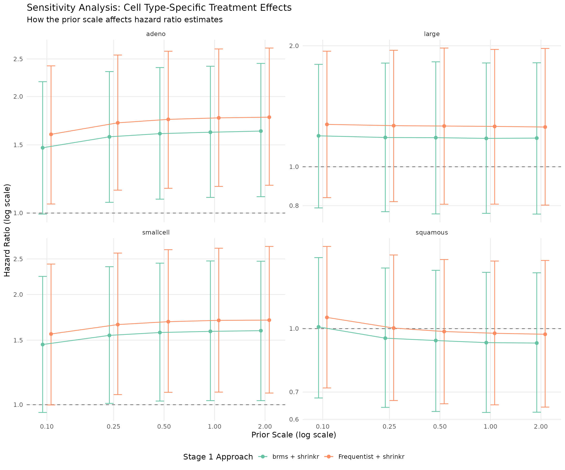
A main advantage of the two-stage framework is that we can explore many hierarchical priors in Stage 2 without refitting the Stage 1 survival model.

prior_summary <- tibble(
  Strength = c("Very Strong", "Strong", "Moderate", "Weak", "Very Weak"),
  Prior = c(
    "Half-Normal(0, 0.1)",
    "Half-Normal(0, 0.25)",
    "Half-Normal(0, 0.5)",
    "Half-Normal(0, 1.0)",
    "Half-Normal(0, 2.0)"
  ),
  Scale = c(0.1, 0.25, 0.5, 1.0, 2.0),
  Interpretation = c(
    "Very similar effects expected",
    "Similar effects expected",
    "Moderate heterogeneity allowed",
    "Substantial differences allowed",
    "Large differences allowed"
  )
)

knitr::kable(prior_summary)

Strength	Prior	Scale	Interpretation
Very Strong	Half-Normal(0, 0.1)	0.10	Very similar effects expected
Strong	Half-Normal(0, 0.25)	0.25	Similar effects expected
Moderate	Half-Normal(0, 0.5)	0.50	Moderate heterogeneity allowed
Weak	Half-Normal(0, 1.0)	1.00	Substantial differences allowed
Very Weak	Half-Normal(0, 2.0)	2.00	Large differences allowed

all_priors <- list(
  very_strong = list(
    mu = dist_normal(0, 1),
    tau = dist_truncated(dist_normal(0, 0.1), lower = 0)
  ),
  strong = list(
    mu = dist_normal(0, 1),
    tau = dist_truncated(dist_normal(0, 0.25), lower = 0)
  ),
  moderate = list(
    mu = dist_normal(0, 1),
    tau = dist_truncated(dist_normal(0, 0.5), lower = 0)
  ),
  weak = list(
    mu = dist_normal(0, 1),
    tau = dist_truncated(dist_normal(0, 1.0), lower = 0)
  ),
  very_weak = list(
    mu = dist_normal(0, 1),
    tau = dist_truncated(dist_normal(0, 2.0), lower = 0)
  )
)

# --- brms fits ---
sensitivity_fits_brms <- lapply(all_priors, function(prior) {
  shrink(
    mixture = mix_brms,
    hierarchical_priors = prior,
    chains = 4,
    iter = 4000,
    warmup = 1000
  )
})

# --- frequentist fits ---
sensitivity_fits_freq <- lapply(all_priors, function(prior) {
  shrink(
    mle = trt_effects,
    var_matrix = trt_vcov,
    hierarchical_priors = prior,
    chains = 4,
    iter = 4000,
    warmup = 1000
  )
})

# --- summaries ---
sensitivity_summaries <- c(
  purrr::imap(sensitivity_fits_brms, function(fit, nm) {
    summ <- summary(fit)
    list(
      theta_summary = summ$theta,
      mu_tau_summary = summ$mu_tau,
      print_output = capture.output(print(fit))
    )
  }),
  purrr::imap(sensitivity_fits_freq, function(fit, nm) {
    summ <- summary(fit)
    list(
      theta_summary = summ$theta,
      mu_tau_summary = summ$mu_tau,
      print_output = capture.output(print(fit))
    )
  })
)

# --- name them clearly ---
names(sensitivity_summaries) <- c(
  paste0(names(all_priors), "_brms"),
  paste0(names(all_priors), "_freq")
)

Prior densities

tau_seq <- seq(0, 3, length.out = 200)

prior_densities <- lapply(names(prior_specs), function(spec_name) {
  spec <- prior_specs[[spec_name]]
  tibble(
    tau = tau_seq,
    density = dnorm(tau_seq, 0, spec$scale) * 2,
    prior_strength = spec$name,
    scale = spec$scale
  )
}) %>%
  bind_rows() %>%
  mutate(
    prior_strength = factor(prior_strength, levels = c(
      "Very Strong", "Strong", "Moderate", "Weak", "Very Weak"
    ))
  )

ggplot(prior_densities, aes(x = tau, y = density, color = prior_strength)) +
  geom_line(linewidth = 1.2) +
  scale_color_brewer(palette = "RdYlBu", direction = -1) +
  labs(
    title = "Prior Densities for the Heterogeneity Parameter (tau)",
    subtitle = "Half-Normal(0, sigma) priors with increasing scale",
    x = "tau",
    y = "Density",
    color = "Prior Strength"
  ) +
  theme(legend.position = "right")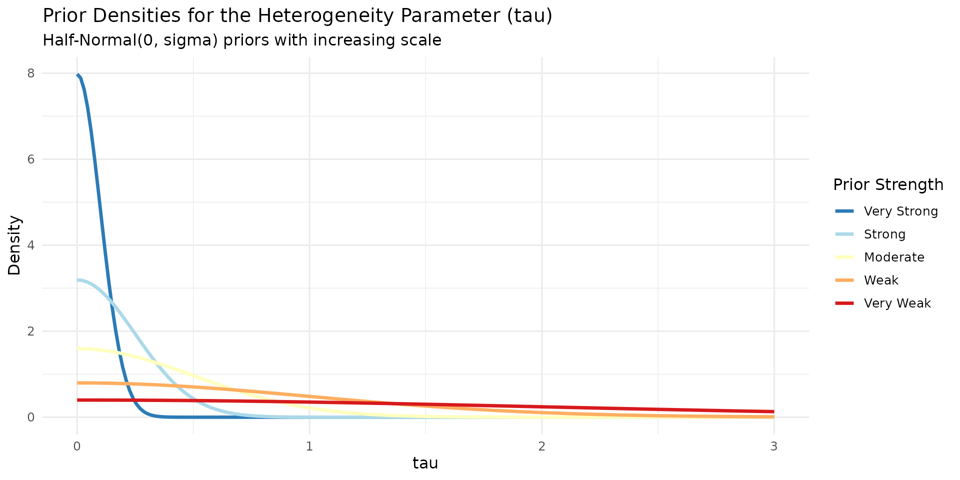

Heterogeneity estimates

tau_results <- lapply(names(sensitivity_summaries), function(fit_name) {
  summary_obj <- sensitivity_summaries[[fit_name]]
  prior_name <- sub("_(brms|freq)$", "", fit_name)
  approach <- if (grepl("_brms$", fit_name)) "brms + shrinkr" else "Frequentist + shrinkr"

  summary_obj$mu_tau_summary %>%
    filter(parameter == "tau") %>%
    mutate(
      prior_strength = prior_specs[[prior_name]]$name,
      prior_scale = prior_specs[[prior_name]]$scale,
      approach = approach
    )
}) %>%
  bind_rows() %>%
  mutate(
    prior_strength = factor(
      prior_strength,
      levels = c("Very Strong", "Strong", "Moderate", "Weak", "Very Weak")
    )
  )

if (all(c("q2.5", "q97.5") %in% names(tau_results))) {
  tau_results <- tau_results %>%
    mutate(lower = `q2.5`, upper = `q97.5`)
} else if (all(c("q5", "q95") %in% names(tau_results))) {
  tau_results <- tau_results %>%
    mutate(lower = q5, upper = q95)
} else {
  stop(
    "Could not find interval columns in sensitivity_summaries$mu_tau_summary. ",
    "Available columns are: ",
    paste(names(tau_results), collapse = ", ")
  )
}

ggplot(tau_results, aes(x = prior_scale, y = mean, color = approach)) +
  geom_point(size = 3, position = position_dodge(width = 0.1)) +
  geom_errorbar(
    aes(ymin = lower, ymax = upper),
    width = 0.1,
    linewidth = 1,
    position = position_dodge(width = 0.1)
  ) +
  geom_line(aes(group = approach), position = position_dodge(width = 0.1)) +
  scale_x_log10(breaks = c(0.1, 0.25, 0.5, 1.0, 2.0)) +
  scale_color_brewer(palette = "Set2") +
  labs(
    title = "Sensitivity of the Heterogeneity Parameter (tau)",
    subtitle = "How prior scale affects the estimated between-cell-type variation",
    x = "Prior Scale (log scale)",
    y = "Posterior tau",
    color = "Stage 1 Approach"
  ) +
  theme(legend.position = "bottom")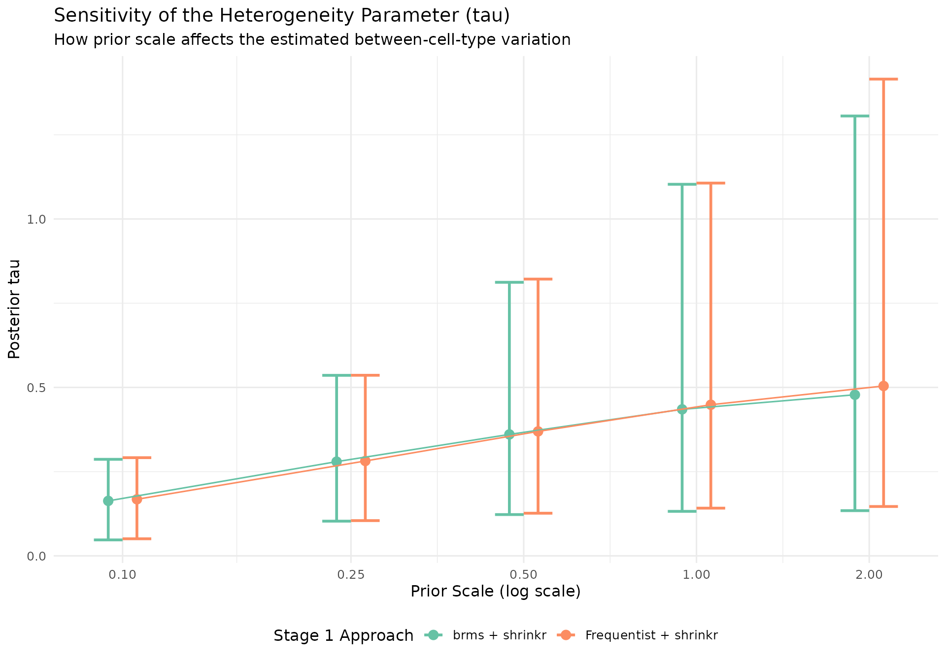

Interpretation:

• Stronger priors constrain tau toward smaller values and produce more shrinkage
• Weaker priors allow more between-cell-type variation
• The posterior for tau stabilizes as the prior becomes less restrictive

Impact on cell type estimates

theta_sensitivity <- lapply(names(sensitivity_summaries), function(fit_name) {
  summary_obj <- sensitivity_summaries[[fit_name]]
  prior_name <- sub("_(brms|freq)$", "", fit_name)
  approach <- if (grepl("_brms$", fit_name)) "brms + shrinkr" else "Frequentist + shrinkr"

  summary_obj$theta_summary %>%
    mutate(
      prior_strength = prior_specs[[prior_name]]$name,
      prior_scale = prior_specs[[prior_name]]$scale,
      approach = approach,
      hr_mean = exp(mean),
      hr_lower = exp(q2.5),
      hr_upper = exp(q97.5)
    )
}) %>%
  bind_rows() %>%
  mutate(
    prior_strength = factor(prior_strength, levels = c(
      "Very Strong", "Strong", "Moderate", "Weak", "Very Weak"
    ))
  )

ggplot(theta_sensitivity, aes(x = prior_scale, y = hr_mean, color = approach)) +
  geom_hline(yintercept = 1, linetype = "dashed", alpha = 0.5) +
  geom_point(size = 2, position = position_dodge(width = 0.1)) +
  geom_errorbar(
    aes(ymin = hr_lower, ymax = hr_upper),
    width = 0.1,
    position = position_dodge(width = 0.1)
  ) +
  geom_line(aes(group = approach), position = position_dodge(width = 0.1)) +
  facet_wrap(~group, ncol = 2, scales = "free_y") +
  scale_x_log10(breaks = c(0.1, 0.25, 0.5, 1.0, 2.0)) +
  scale_y_log10() +
  scale_color_brewer(palette = "Set2") +
  labs(
    title = "Sensitivity Analysis: Cell Type-Specific Treatment Effects",
    subtitle = "How the prior scale affects hazard ratio estimates",
    x = "Prior Scale (log scale)",
    y = "Hazard Ratio (log scale)",
    color = "Stage 1 Approach"
  ) +
  theme(
    legend.position = "bottom",
    panel.grid.minor = element_blank()
  )

Key Takeaways

1. The two-stage brms + shrinkr workflow closely matches the full hierarchical brms analysis in this example.
2. The two-stage approach is modular: fit the survival model once, then explore many hierarchical priors efficiently.
3. Sensitivity analysis becomes straightforward because Stage 2 can be rerun without refitting Stage 1.
4. fit_mixture() provides a flexible approximation to the subgroup posteriors, and shrink() adds hierarchical regularization on top of that approximation.

Session Info

sessionInfo()
#> R version 4.6.1 (2026-06-24)
#> Platform: x86_64-pc-linux-gnu
#> Running under: Ubuntu 24.04.4 LTS
#> 
#> Matrix products: default
#> BLAS:   /usr/lib/x86_64-linux-gnu/openblas-pthread/libblas.so.3 
#> LAPACK: /usr/lib/x86_64-linux-gnu/openblas-pthread/libopenblasp-r0.3.26.so;  LAPACK version 3.12.0
#> 
#> locale:
#>  [1] LC_CTYPE=C.UTF-8       LC_NUMERIC=C           LC_TIME=C.UTF-8       
#>  [4] LC_COLLATE=C.UTF-8     LC_MONETARY=C.UTF-8    LC_MESSAGES=C.UTF-8   
#>  [7] LC_PAPER=C.UTF-8       LC_NAME=C              LC_ADDRESS=C          
#> [10] LC_TELEPHONE=C         LC_MEASUREMENT=C.UTF-8 LC_IDENTIFICATION=C   
#> 
#> time zone: UTC
#> tzcode source: system (glibc)
#> 
#> attached base packages:
#> [1] stats     graphics  grDevices utils     datasets  methods   base     
#> 
#> other attached packages:
#>  [1] patchwork_1.3.2      posterior_1.7.0      survival_3.8-6      
#>  [4] lubridate_1.9.5      forcats_1.0.1        stringr_1.6.0       
#>  [7] dplyr_1.2.1          purrr_1.2.2          readr_2.2.0         
#> [10] tidyr_1.3.2          tibble_3.3.1         ggplot2_4.0.3       
#> [13] tidyverse_2.0.0      distributional_0.8.1 tidybayes_3.0.7     
#> [16] brms_2.23.0          Rcpp_1.1.1-1.1       shrinkr_0.4.5       
#> 
#> loaded via a namespace (and not attached):
#>  [1] tidyselect_1.2.1      svUnit_1.0.8          farver_2.1.2         
#>  [4] loo_2.10.0            S7_0.2.2              fastmap_1.2.0        
#>  [7] tensorA_0.36.2.1      digest_0.6.39         timechange_0.4.0     
#> [10] lifecycle_1.0.5       StanHeaders_2.32.10   magrittr_2.0.5       
#> [13] compiler_4.6.1        rlang_1.2.0           sass_0.4.10          
#> [16] tools_4.6.1           utf8_1.2.6            yaml_2.3.12          
#> [19] knitr_1.51            labeling_0.4.3        bridgesampling_1.2-1 
#> [22] htmlwidgets_1.6.4     pkgbuild_1.4.8        mclust_6.1.2         
#> [25] RColorBrewer_1.1-3    abind_1.4-8           withr_3.0.3          
#> [28] desc_1.4.3            grid_4.6.1            stats4_4.6.1         
#> [31] inline_0.3.21         scales_1.4.0          cli_3.6.6            
#> [34] mvtnorm_1.4-1         rmarkdown_2.31        ragg_1.5.2           
#> [37] generics_0.1.4        otel_0.2.0            RcppParallel_5.1.11-2
#> [40] tzdb_0.5.0            cachem_1.1.0          rstan_2.32.7         
#> [43] splines_4.6.1         bayesplot_1.15.0      parallel_4.6.1       
#> [46] matrixStats_1.5.0     vctrs_0.7.3           Matrix_1.7-5         
#> [49] jsonlite_2.0.0        hms_1.1.4             arrayhelpers_1.1-0   
#> [52] systemfonts_1.3.2     ggdist_3.3.3          jquerylib_0.1.4      
#> [55] glue_1.8.1            pkgdown_2.2.0         codetools_0.2-20     
#> [58] stringi_1.8.7         gtable_0.3.6          QuickJSR_1.10.0      
#> [61] pillar_1.11.1         htmltools_0.5.9       Brobdingnag_1.2-9    
#> [64] R6_2.6.1              textshaping_1.0.5     evaluate_1.0.5       
#> [67] lattice_0.22-9        backports_1.5.1       bslib_0.11.0         
#> [70] rstantools_2.6.0      coda_0.19-4.1         gridExtra_2.3.1      
#> [73] nlme_3.1-169          checkmate_2.3.4       xfun_0.59            
#> [76] fs_2.1.0              pkgconfig_2.0.3