Getting Started with multigrain

What Does `multigrain` Do?

The multigrain package is designed to optimise graph-based multiple testing procedures by identifying the hypothesis and transition weights that maximise a user-defined definition of trial success, given an expected distribution of test statistics.

A graphical test has:

An $m$ -length hypothesis weight vector ( $w$ ), which determines how $\alpha$ is initially allocated between hypotheses in the graph.
A transition matrix ( $\mathbf{G}$ ) of dimensions $m \times m$ which determines how $\alpha$ can be recycled from a null hypothesis after it has been rejected to other unrejected hypotheses.

Optimising for different power metrics or trial success criteria will often lead to distinct graphs, i.e., distinct values for the parameters that make up the hypothesis weight vectors ( $w$ ), and the transition matrices ( $\mathbf{G}$ ).

Each trial success measure has its own optimal configuration of these parameters that maximizes the desired success criterion. The multigrain function graph_optimise() is the tool that identifies these optimal parameters, enabling users to find the graph that gives that highest value for their chosen trial success measure.

Motivating Example

Consider a two-arm parallel confirmatory clinical trial to compare a high and low dose of an investigational treatment in patients with asthma versus placebo.

There are two endpoints included in the multiplicity adjustment:

a primary endpoint, FEV1;
a secondary endpoint, a patient-report outcome (PRO).

Thus there are four hypotheses, the primary hypotheses $H_1$ and $H_2$ on FEV1 comparing high and low dose of the investigational treatment against placebo, and the secondary hypotheses $H_3$ and $H_4$ on the PRO endpoint for the high and low dose comparisons against placebo.

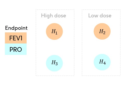
Figure 1: Hypotheses for asthma motivating example

The secondary hypothesis for the PRO endpoint will only be tested after the corresponding primary endpoint FEV1 has been rejected for the same dose.

Inputs for optimisation by `multigrain`

Optimisation of graphical tests is conducted using the function graph_optimise() from the multigrain package.

In order to optimise a graph-based multiple testing procedure, we require three things:

P-value matrix approximating joint distribution of p-values
A trial success measure
Required constraints on a graph

P-value matrix approximating the joint distribution of p-values

graph_optimise() expects a matrix $\mathbf{P}$ of raw p-values with dimension $n_{\text{sim}}\times m$ .

Each row $i$ is a simulation of p-values from the $m$ null hypotheses $H_1, H_2, ..., H_m$ under the alternative hypothesis that configuration you wish to evaluate.

There are two equivalent ways to provide $\mathbf{P}$ :

Supply your own p-value matrix (e.g., from end-to-end trial simulation).
Generate $\mathbf{P}$ with simulate_pvalues(), which uses the standard normal-approximation for one-sided test statistics (described next).

From the joint test statistic distribution to p-value matrix

At the design stage it is common to assume the one-sided test statistics are jointly normal:

$\boldsymbol{Z} \sim \mathrm{MVN}(\boldsymbol{\Delta}, \boldsymbol{\Sigma}),$

where:

$\boldsymbol{\Delta}$ are the non-centrality parameters (NCPs) reflecting the standardised effect sizes,
$\boldsymbol{\Sigma}$ is the correlation matrix describing the dependence between the test statistics.

Each “raw” p-value (a p-value unadjusted for multiplicity) arises from the transformation:

$p_i = 1 - \operatorname{\Phi}(z_i)$

so the p-values inherit a joint distribution determined entirely by $(\boldsymbol{\Delta}, \boldsymbol{\Sigma})$ .

Often you know the one-sided nominal per-hypothesis power (the power of each hypothesis unadjusted for multiplicity) - $\pi_i = 1 - \beta_i$ - at level $\alpha$ , rather than the non-centrality parameter $\Delta_i$ . There is a one-to-one relationship between $\pi_i$ and $\Delta_i$ :

$\Delta_i \;=\; \Phi^{-1}(1-\alpha)\;-\;\Phi^{-1}(1-\pi_i).$

[simulate_pvalues()] performs this conversion internally, simulates $\boldsymbol{Z}\sim\mathrm{MVN}(\boldsymbol{\Delta},\boldsymbol{\Sigma})$ , and returns raw p-values $p_i=1-\Phi(Z_i)$ to generate a matrix of nsim simulations.

Important: Note on One-Sided Tests and Power Terminology

One-Sided Tests and Power Terminology

When designing and optimising a graph, it’s essential to use a one-sided testing framework. The simulation engine in multigrain is built on a model of one-sided test statistics, assuming $z \sim \mathrm{MVN}(\boldsymbol{\Delta}, \boldsymbol{\Sigma})$ , to correctly represent the direction of a treatment’s effect. For this reason, you should specify a one-sided alpha level (e.g., $\alpha = 0.025$ , which is also the default being used).

Power Terminology

Furthermore, the term for the input power vector (power_nominal in simulate_pvalues()) can be a point of confusion. We use the term nominal per-hypothesis power to refer to the power of each hypothesis before any multiplicity adjustment, as if it were tested in isolation at the full alpha level. This is distinct from the local power, which is the actual probability of rejecting a hypothesis after the graphical procedure is applied.

Asthsma example: simulating the p-value matrix using `simulate_pvalues()`

with working correlation matrix for $(H_1,\dots,H_4)$ :

$\boldsymbol{\Sigma} = \begin{bmatrix} 1 & 0.5 & 0.8 & 0.4 \\ 0.5 & 1 & 0.4 & 0.8 \\ 0.8 & 0.4 & 1 & 0.5 \\ 0.4 & 0.8 & 0.5 & 1 \end{bmatrix}.$

power_vector <- c(0.97, 0.91, 0.86, 0.83)
corr_matrix <- matrix(
  c(1, 0.5, 0.8, 0.4,
    0.5, 1, 0.4, 0.8,
    0.8, 0.4, 1, 0.5,
    0.4, 0.8, 0.5, 1),
  nrow = 4, byrow = TRUE
)

set.seed(1)
pvals <- simulate_pvalues(
    power_nominal = power_vector,
    alpha = 0.025,
    corr_matrix = corr_matrix,
    nsim = 1e6 # Increase for greater precision
)

dim(pvals) # n.sim × 4
#> [1] 1000000       4
head(pvals) # first few rows
#>              [,1]         [,2]         [,3]         [,4]
#> [1,] 7.734878e-04 4.677161e-05 7.378574e-03 2.015044e-05
#> [2,] 1.160596e-05 1.169174e-03 1.167596e-04 4.061633e-04
#> [3,] 3.422976e-07 2.210753e-04 1.659601e-06 2.034029e-04
#> [4,] 5.337848e-04 8.781843e-02 2.534725e-04 1.755350e-02
#> [5,] 3.933848e-06 4.022113e-06 3.310420e-05 2.870895e-05
#> [6,] 1.939926e-06 4.212138e-04 8.690317e-04 4.876759e-02

Trial Success Measure

The trial success measure is the target quantity that graph_optimise() maximises. It encodes the success criteria for a trial by mapping the outcomes of the graphical test to a numerical score. (A dedicated vignette on trial success measures is planned for a future release.)

After analyzing the collected data from our trial, we obtain four raw p-values: $p_1, p_2, p_3, p_4$ , each corresponding to one of our hypotheses $H_1, H_2, H_3, H_4$ .

Our output after applying our graphical test to our p-values will be a binary rejection vector:

$\boldsymbol{r} = (r_1, r_2, r_3, r_4)$

where $r_i = 1$ if $H_i$ is rejected, and $0$ otherwise.

The trial success measure is then defined as the expected value of a user-specified function of $\boldsymbol{r}$ . In our asthma example, we will use two different examples of trial success measures:

Average Power: This measures the mean proportion of hypotheses rejected across trials: $\text{Average Power} = \mathbb{E} \left[ \frac{1}{4} ( r_1 + r_2 + r_3 + r_4 ) \right]$
Custom Trial Success: In our example, it seems natural to declare a trial successful if at least one of the two primary dose-control comparisons ( $H_1$ or $H_2$ ) is statistically significant. Rejecting a key secondary ( $H_3$ or $H_4$ ) would be ‘nice to have,’ but not essential for claiming the success of a trial. It also seems natural that we should not ascribe additional benefit for rejecting a secondary hypothesis without having first rejected the associated primary hypothesis for the same dose. Therefore we can construct the following power objective for our example:
- Success for rejecting at least one of the two primary dose-control comparisons $H_1$ or $H_2$ (but no extra credit for rejecting both)
- $H_3$ and $H_4$ only add value if their corresponding primary endpoints ( $H_1$ and $H_2$ ) are also rejected.

$\text{Custom Trial Success} = \mathbb{E} \left[ \frac{1}{4} \left( 2 \times \mathbb{I}(r_1 + r_2 \geq 1) + r_1 \times r_3 + r_2 \times r_4 \right) \right]$ where: $\mathbb{I}(r_1 + r_2 \geq 1) = \begin{cases} 1, & \text{if } r_1 \text{ or } r_2 = 1 \\ 0, & \text{otherwise} \end{cases}$

Implementing trial success measures using `trial_success()`

We can create functions to quickly calculate our trial success measures during graph optimisation by using the trial_success() functions. This function will output a trial_success object, which will contain a function we will use to calculate our custom trial success measure during and after optimisation, allowing us to evaluate the performance of different graphs. trial_success() will write this function in C++ using the Rcpp package.

# Creating power objective functions as targets for optimisation
average_power <- trial_success(0.25 * (r1 + r2 + r3 + r4))
#> ✔ Trial success function compiled and sourced successfully.
custom_trial_success <- trial_success(
    0.25 * (2 * (r1 && r2) + r1 * r3 + r2 * r4)
)
#> ✔ Trial success function compiled and sourced successfully.

Multiplying our objective functions by $0.25$ scale our objective functions so that they are in the interval $[0, 1]$ , but this is not necessary for optimisation.

Constraints on a graph

Let us assume that we decide a priori to avoid testing a secondary hypothesis for a dose-control comparison without having rejected the associated primary hypothesis. We can ensure that the optimal graph is found within this logical constraint by using the graph_constraint() function.

# Creating a graph constraint object to enforce logical constraints
# on order of rejections

hyp_constraint <- c(NA, NA, 0, 0)
trans_constraint <- matrix(
  c(0, NA, NA, 0,
    NA, 0, 0, NA,
    0, 1, 0, 0,
    1, 0, 0, 0),
  nrow = 4,
  byrow = TRUE
)

my_constraint <- graph_constraint(
    hyp_constraint = hyp_constraint,
    trans_constraint = trans_constraint
)

print(my_constraint)
#> <multigrain_graph_constraint>
#> Constraints on hypothesis weights:
#> H1 H2 H3 H4 
#> NA NA  0  0 
#> 
#> Constraints on transition matrix:
#>    H1 H2 H3 H4
#> H1  0 NA NA  0
#> H2 NA  0  0 NA
#> H3  0  1  0  0
#> H4  1  0  0  0

NA signifies “no constraint”, i.e., the hypothesis weight or transition weight can take any value within $[0, 1]$ (as long as the hypothesis weights or sum of the transition matrix rows sum to 1).
If a weight vector or matrix element contains a number (e.g., 1), it means means the corresponding hypothesis or transition weight is fixed and will not be optimised.
A zero as an element in the transition matrix means no (initial) edge is allowed between the corresponding hypotheses.
All diagonals must be zero in the transition matrix (as alpha must be propagated) to other hypotheses after rejection.

The above code leads to the following general graph:

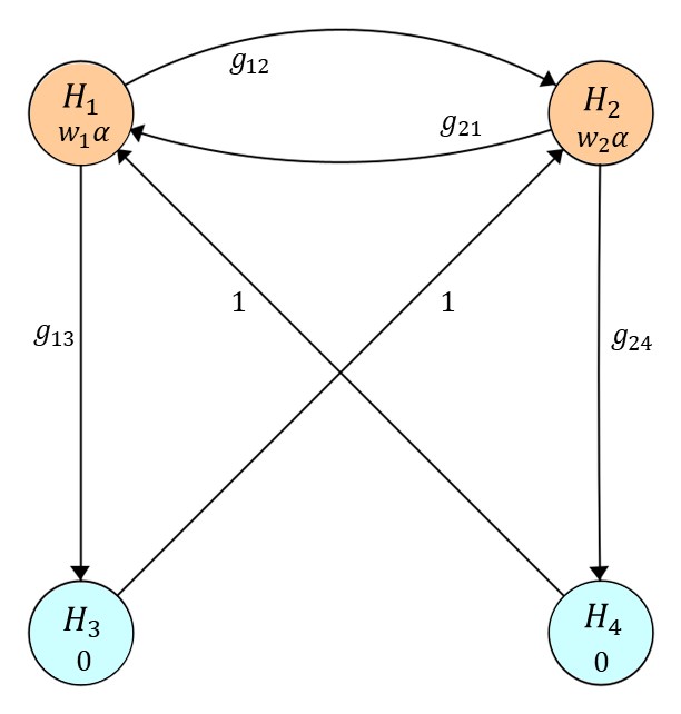
Figure 2: Graph with constraints for “Getting Started with multigrain” asthma example

Only the hypothesis weights $w_1, w_2$ and transition weights $g_{12}, g_{21}, g_{13}, g_{24}$ will be optimised.

Although not necessary, setting constraints on a graph can speed up the optimisation since we will have less parameters to optimise.

We can check the constraints using plot(my_constraint) (see below):

plot(my_constraint)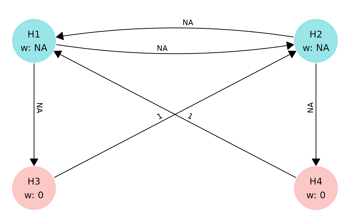

Please see the dedicated vignette on this topic for more details about setting and plotting graph constraints.

Optimising the graph

Now we have our inputs (assumed test statistic distribution, a trial_success object containing our function to quickly calculate the trial success measure, and optional constraints on the graph), we are ready to optimise using graph_optimise(). We will optimise for our two objective functions, average_power and custom_trial_success separately.

# Find optimal graph based on average power objective function
graph_average_power <- graph_optimise(
    pvals = pvals,
    graph_constraint = my_constraint,
    alpha = 0.025, # one-sided
    trial_success = average_power
)

# Find optimal graph based on custom power objective function (defined earlier)
graph_custom_trial_success <- graph_optimise(
    pvals = pvals,
    graph_constraint = my_constraint,
    alpha = 0.025, # one-sided
    trial_success = custom_trial_success
)

Important: Tuning the optimiser for precision vs. speed (click to reveal)

Tuning the Optimiser for Precision vs. Speed

The back-end of graph_optimise() executes two searches in sequence:

a global search of the solution space using a genetic algorithm;
a local “hill-climbing” algorithm (COBYLA) that refines the best region found by the global search.

All tuning is done through a multigrain_control() object, which is passed to graph_optimise() via the control argument.

Number of simulations

control_nsim_global() and control_nsim_local() set the number of p-value rows used to evaluate trial success during the global and local phases respectively:

ctrl <- multigrain_control() |>
  control_nsim_global(50000) |>
  control_nsim_local(500000)

We recommend at least 50,000 simulations for the global search if the graph will be used in a protocol/SAP.
The local search should use as many simulations as possible (at least 500,000). By default graph_optimise() uses all rows of the pvals matrix you provide.

Stopping the global search

The global search (genetic algorithm) stops after the trial success measure fails to improve for a number of consecutive generations. This is controlled by the run parameter (from GA::ga()), accessible via control_global():

ctrl <- ctrl |>
  control_global(run = 1000)

The default is 200 generations, which returns a graph quickly.
For a graph that will be used in a protocol/SAP, set run to at least 1000 to ensure a thorough search.

Parallel execution

For large problems with many hypotheses (m ≥ 6), enable parallel execution via the num_threads argument of graph_optimise():

g_opt <- graph_optimise(
  pvals = pvals,
  graph_constraint = my_constraint,
  alpha = 0.025,
  trial_success = custom_trial_success,
  num_threads = 4
)

Skipping the global search

Additionally, if you already have a good starting graph, you can skip the global search entirely by setting global_search to FALSE:

g_opt <- graph_optimise(
  pvals = pvals,
  graph_constraint = my_constraint,
  alpha = 0.025,
  trial_success = custom_trial_success,
  global_search = FALSE,
  num_threads = 4
)

Putting it together

ctrl <- multigrain_control() |>
  control_nsim_global(50000) |>
  control_nsim_local(1e6) |>
  control_global(run = 1000)

g_opt <- graph_optimise(
  pvals = pvals,
  graph_constraint = my_constraint,
  alpha = 0.025,
  trial_success = custom_trial_success,
  num_threads = 4,
  control = ctrl
)

Results

Once optimised, we can retrieve a summary from the optimal_graph objects produced by graph_optimise():

print(
    "Summary of the optimisation results for the graph optimised for AVERAGE power"
)
summary(graph_average_power)

#> [1] "Summary of the optimisation results for the graph optimised for AVERAGE power"
#> <multigrain_graph_optimal>
#> Optimal graph found (given user-defined constraints on graph and computational resources):
#> 
#> Hypothesis weights:
#>     H1     H2     H3     H4 
#> 0.7697 0.2303 0.0000 0.0000 
#> 
#> Transition matrix:
#>    H1     H2     H3 H4
#> H1  0 0.4089 0.5911  0
#> H2  0 0.0000 0.0000  1
#> H3  0 1.0000 0.0000  0
#> H4  1 0.0000 0.0000  0
#> 
#> Trial success function:
#> 0.25 * (r1 + r2 + r3 + r4)
#> 
#> Value of trial success measure:
#> 0.863
#> [1] "Summary of the optimisation results for the graph optimised for CUSTOM power"
#> <multigrain_graph_optimal>
#> Optimal graph found (given user-defined constraints on graph and computational resources):
#> 
#> Hypothesis weights:
#>     H1     H2     H3     H4 
#> 0.9925 0.0075 0.0000 0.0000 
#> 
#> Transition matrix:
#>        H1     H2     H3     H4
#> H1 0.0000 0.7963 0.2037 0.0000
#> H2 0.5903 0.0000 0.0000 0.4097
#> H3 0.0000 1.0000 0.0000 0.0000
#> H4 1.0000 0.0000 0.0000 0.0000
#> 
#> Trial success function:
#> 0.25 * (2 * (r1 && r2) + r1 * r3 + r2 * r4)
#> 
#> Value of trial success measure:
#> 0.8391

We can plot the graph using the plot() function for the optimal_graph objects.

p1 <- plot(graph_average_power) +
    ggtitle("Optimal Graph for Average Power") +
    theme(
        plot.title = element_text(
            hjust = 0.5,
            size = 14,
            margin = margin(0, 0, 30, 0)
        )
    )

p2 <- plot(graph_custom_trial_success) +
    ggtitle("Optimal Graph for Custom Success") +
    theme(
        plot.title = element_text(
            hjust = 0.5,
            size = 14,
            margin = margin(0, 0, 30, 0)
        )
    )

gridExtra::grid.arrange(p1, p2, ncol = 2)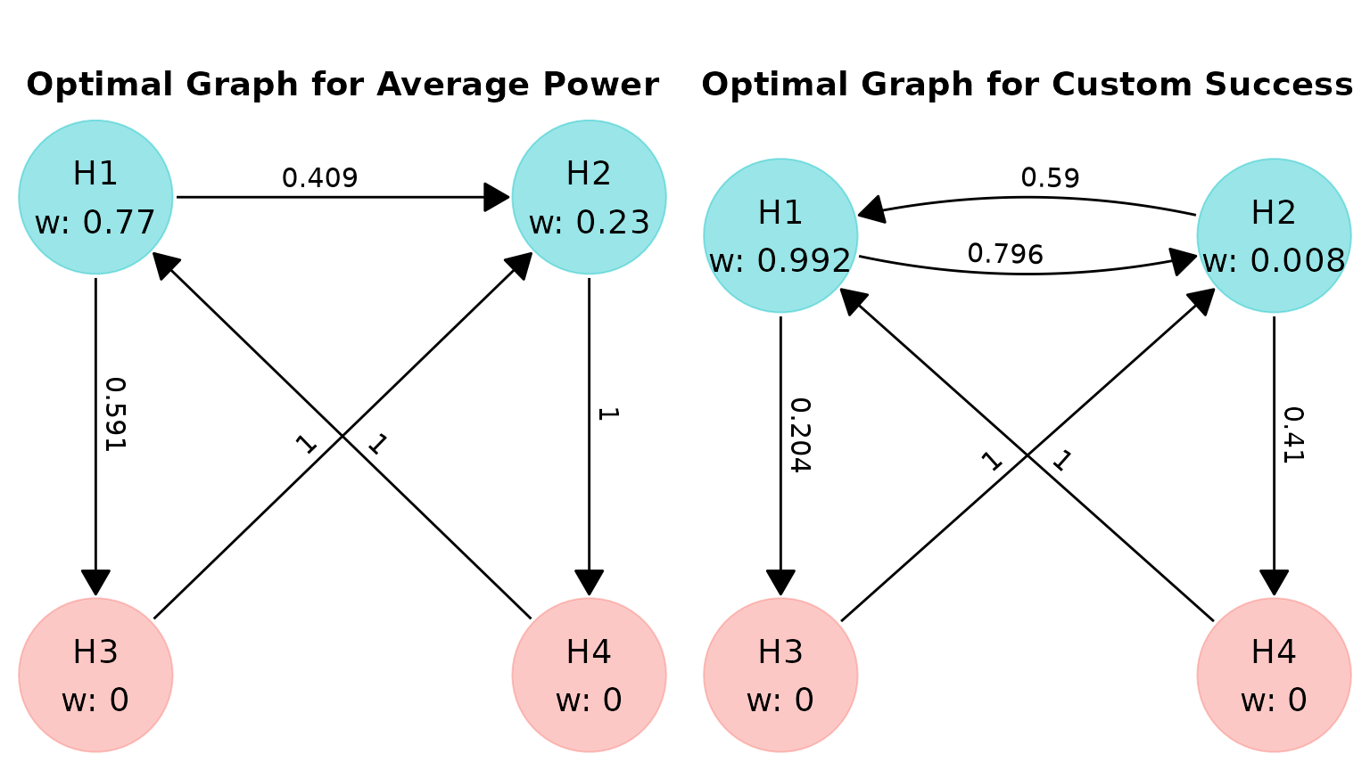

Evaluating Trial Success

We can evaluate the power / trial success of each graph by using the calc_power_pvals() function.

# Calculate power for graph optimised for average power
graph_avg_power_metrics <- calc_power_pvals(
    pvals,
    alpha = 0.025,
    hyp_weight = graph_average_power$hyp_weight,
    trans_matrix = graph_average_power$trans_matrix,
    custom_power = list("CustomSuccess" = custom_trial_success)
)

# Expected Rejections / 4 is equal to average power
print(graph_avg_power_metrics)
#> $local_power
#> [1] 0.963991 0.886115 0.821594 0.779022
#> 
#> $exp_rejections
#> [1] 3.450722
#> 
#> $disj_power
#> [1] 0.975687
#> 
#> $conj_power
#> [1] 0.720786
#> 
#> $CustomSuccess
#> [1] 0.8373635

# Calculate power for graph optimised for custom power metric
graph_custom_ts_metrics <- calc_power_pvals(
    pvals,
    alpha = 0.025,
    hyp_weight = graph_custom_trial_success$hyp_weight,
    trans_matrix = graph_custom_trial_success$trans_matrix,
    custom_power = list("CustomSuccess" = custom_trial_success)
)

# Expected Rejections / 4 is equal to average power
print(graph_custom_ts_metrics)
#> $local_power
#> [1] 0.969727 0.886183 0.807867 0.777944
#> 
#> $exp_rejections
#> [1] 3.441721
#> 
#> $disj_power
#> [1] 0.971455
#> 
#> $conj_power
#> [1] 0.721501
#> 
#> $CustomSuccess
#> [1] 0.8386803

Graph	H1	H2	H3	H4	Average Power	Custom Success
Optimised for AvgPower	0.964	0.886	0.822	0.779	0.863	0.837
Optimised for CustomPower	0.970	0.886	0.808	0.778	0.860	0.839

In the table above:

Columns H1 - H4 show the local power of each hypothesis under the graph and the assumed test statistic distribution,
Average Power and Custom Success show the value of the objective functions defined in the section on trial success measures.

What Does multigrain Do?